.ipynb .pdf

repository open issue

Binder

Contents

Lab 2: Cluster analysis of sequential data

About the dataset

In this lab, we are going to use the built-in biofam data set from the TraMineR package. See more details here

This data consists information about the Family life states from the Swiss Household Panel biographical survey. 16 year-long family life sequences built from the retrospective biographical survey carried out by the Swiss Household Panel (SHP) in 2002.

A data frame with 2000 rows, 16 state variables, 1 id variable and 7 covariates and 2 weights variables.

The data set contains (in columns 10 to 25) sequences of family life states from age 15 to 30 (sequence length is 16) and a series of covariates. The sequences are a sample of 2000 sequences of those created from the SHP biographical survey. It includes only individuals who were at least 30 years old at the time of the survey. The biofam data set describes family life courses of 2000 individuals born between 1909 and 1972.

The states numbered from 0 to 7 are defined from the combination of five basic states, namely Living with parents (Parent), Left home (Left), Married (Marr), Having Children (Child), Divorced:

0 = “Parent”
1 = “Left”
2 = “Married”
3 = “Left+Marr”
4 = “Child”
5 = “Left+Child”
6 = “Left+Marr+Child”
7 = “Divorced”

Variable	Label
idhous	ID
sex	sex
birthy	birth year
nat102	nationality
plingu02	interview language
p02r01	confession or religion
p02r04	participation in religious services: frequency
cspfaj	Swiss socio-professional category: Fathers job
cspmoj	Swiss socio-professional category: Mothers job
a15	family status at age 15
…
a30	family status at age 30

library(tidyverse)
library(TraMineR)
library(cluster)
data(biofam)
str(biofam)

── Attaching packages ──────────────────────────────────────────────────────────────────────────── tidyverse 1.3.1 ──

✔ ggplot2 3.3.5     ✔ purrr   0.3.4
✔ tibble  3.1.5     ✔ dplyr   1.0.7
✔ tidyr   1.1.3     ✔ stringr 1.4.0
✔ readr   2.0.1     ✔ forcats 0.5.1

Warning message:
“package ‘tibble’ was built under R version 4.1.1”

Warning message:
“package ‘readr’ was built under R version 4.1.1”

── Conflicts ─────────────────────────────────────────────────────────────────────────────── tidyverse_conflicts() ──
✖ dplyr::filter() masks stats::filter()
✖ dplyr::lag()    masks stats::lag()

Warning message:
“package ‘TraMineR’ was built under R version 4.1.1”

TraMineR stable version 2.2-3 (Built: 2022-01-26)

Website: http://traminer.unige.ch

Please type 'citation("TraMineR")' for citation information.

Warning message:
“package ‘cluster’ was built under R version 4.1.1”

'data.frame':	2000 obs. of  27 variables:
 $ idhous  : num  66891 28621 57711 17501 147701 ...
 $ sex     : Factor w/ 2 levels "man","woman": 1 1 2 1 1 1 1 1 1 2 ...
 $ birthyr : num  1943 1935 1946 1918 1946 ...
 $ nat_1_02: Factor w/ 200 levels "other error",..: 6 6 6 6 6 6 6 6 6 6 ...
 $ plingu02: Factor w/ 3 levels "french","german",..: 2 2 1 2 2 3 2 1 1 2 ...
 $ p02r01  : Factor w/ 13 levels "other error",..: 6 7 13 7 7 7 6 9 6 7 ...
 $ p02r04  : Factor w/ 14 levels "other error",..: 9 13 7 13 7 6 7 14 9 13 ...
 $ cspfaj  : Factor w/ 12 levels "active occupied but not classified",..: 7 7 7 5 NA 12 NA 11 7 7 ...
 $ cspmoj  : Factor w/ 12 levels "active occupied but not classified",..: 7 NA 9 NA NA NA NA NA 7 NA ...
 $ a15     : num  0 0 0 0 0 0 0 0 0 1 ...
 $ a16     : num  0 1 0 0 0 0 0 0 0 1 ...
 $ a17     : num  0 1 0 0 0 0 0 0 0 1 ...
 $ a18     : num  0 1 0 0 0 0 0 0 0 1 ...
 $ a19     : num  0 1 0 0 0 0 0 0 0 1 ...
 $ a20     : num  0 1 0 1 1 0 0 0 0 1 ...
 $ a21     : num  0 1 0 1 1 0 0 1 0 1 ...
 $ a22     : num  0 1 1 1 1 0 0 1 0 1 ...
 $ a23     : num  0 1 1 1 1 0 0 1 0 1 ...
 $ a24     : num  3 1 1 1 1 0 2 1 0 6 ...
 $ a25     : num  6 1 1 1 1 0 2 1 0 6 ...
 $ a26     : num  6 3 1 1 1 0 2 3 6 6 ...
 $ a27     : num  6 6 3 1 1 0 2 3 6 6 ...
 $ a28     : num  6 6 6 1 6 0 2 3 6 6 ...
 $ a29     : num  6 6 6 1 6 0 2 6 6 6 ...
 $ a30     : num  6 6 6 1 6 0 2 6 6 6 ...
 $ wp00tbgp: num  1053 855 575 1527 796 ...
 $ wp00tbgs: num  0.935 0.759 0.51 1.356 0.707 ...

# state labels
bfstates <- c("Parent", "Left", "Married", "Left+Marr", "Child", "Left+Child", "Left+Marr+Child", "Divorced")

# define sequence object
biofam.seq <- seqdef(biofam, 10:25, states = bfstates, labels = bfstates)

 [>] state coding:

       [alphabet]  [label]         [long label] 

     1  0           Parent          Parent

     2  1           Left            Left

     3  2           Married         Married

     4  3           Left+Marr       Left+Marr

     5  4           Child           Child

     6  5           Left+Child      Left+Child

     7  6           Left+Marr+Child Left+Marr+Child

     8  7           Divorced        Divorced

 [>] 2000 sequences in the data set

 [>] min/max sequence length: 16/16

Q1. Create a normalized dissimilarity matrix using Longest Common Subsequences method

Store the dissimilarity matrix in biofam.seq.LCS

biofam.seq.LCS <- NULL

# BEGIN SOLUTION
biofam.seq.LCS <- seqdist(biofam.seq, method='LCS', norm = 'auto')
biofam.seq.LCS

# END SOLUTION

 [>] 2000 sequences with 8 distinct states

 [>] creating a 'sm' with a substitution cost of 2

 [>] creating 8x8 substitution-cost matrix using 2 as constant value

 [>] 537 distinct  sequences 

 [>] min/max sequence lengths: 16/16

 [>] computing distances using the LCS gmean normalized metric

 [>] elapsed time: 0.214 secs

A matrix: 2000 × 2000 of type dbl

	1167	514	1013	275	2580	773	1187	47	2091	1846	⋯	278	1980	787	1120	59	629	2297	775	2522	719
1167	0.0000	0.6250	0.3125	0.6875	0.5000	0.4375	0.4375	0.4375	0.1250	0.6250	⋯	0.4375	0.6875	0.4375	0.3750	0.4375	0.2500	0.5625	0.4375	0.8125	0.2500
514	0.6250	0.0000	0.3750	0.3125	0.2500	0.9375	0.9375	0.4375	0.6875	0.1875	⋯	0.9375	0.3125	0.8125	0.8750	0.9375	0.5000	0.2500	0.9375	0.9375	0.6875
1013	0.3125	0.3750	0.0000	0.3750	0.1875	0.5625	0.5625	0.1250	0.3750	0.5000	⋯	0.5625	0.3750	0.4375	0.5000	0.5625	0.2500	0.3125	0.5625	0.8125	0.4375
275	0.6875	0.3125	0.3750	0.0000	0.1875	0.6875	0.6875	0.3750	0.6875	0.4375	⋯	0.6875	0.0000	0.5625	0.6875	0.6875	0.5000	0.5000	0.6875	0.8125	0.6875
2580	0.5000	0.2500	0.1875	0.1875	0.0000	0.6875	0.6875	0.2500	0.5000	0.3125	⋯	0.6875	0.1875	0.5625	0.6250	0.6875	0.3125	0.3125	0.6875	0.8125	0.5000
773	0.4375	0.9375	0.5625	0.6875	0.6875	0.0000	0.4375	0.6250	0.3125	1.0000	⋯	0.0000	0.6875	0.1250	0.0625	0.1875	0.6250	0.8750	0.0000	0.8125	0.6250
1187	0.4375	0.9375	0.5625	0.6875	0.6875	0.4375	0.0000	0.6250	0.4375	1.0000	⋯	0.4375	0.6875	0.4375	0.4375	0.2500	0.6250	0.8750	0.4375	0.3750	0.6250
47	0.4375	0.4375	0.1250	0.3750	0.2500	0.6250	0.6250	0.0000	0.5000	0.5625	⋯	0.6250	0.3750	0.5000	0.5625	0.6250	0.3125	0.2500	0.6250	0.8125	0.5000
2091	0.1250	0.6875	0.3750	0.6875	0.5000	0.3125	0.4375	0.5000	0.0000	0.6875	⋯	0.3125	0.6875	0.3125	0.2500	0.3125	0.3125	0.6250	0.3125	0.8125	0.3125
1846	0.6250	0.1875	0.5000	0.4375	0.3125	1.0000	1.0000	0.5625	0.6875	0.0000	⋯	1.0000	0.4375	0.8750	0.9375	1.0000	0.3750	0.3750	1.0000	1.0000	0.5625
1990	0.4375	0.8750	0.5000	0.6875	0.6875	0.5000	0.5000	0.4375	0.5000	1.0000	⋯	0.5000	0.6875	0.5000	0.5000	0.5000	0.6250	0.6250	0.5000	0.8125	0.6250
2088	0.4375	0.9375	0.5625	0.6875	0.6875	0.0000	0.4375	0.6250	0.3125	1.0000	⋯	0.0000	0.6875	0.1250	0.0625	0.1875	0.6250	0.8750	0.0000	0.8125	0.6250
867	0.2500	0.3750	0.1875	0.4375	0.2500	0.6875	0.6875	0.2500	0.3750	0.3750	⋯	0.6875	0.4375	0.5625	0.6250	0.6875	0.1250	0.3125	0.6875	0.8125	0.3125
1616	0.2500	0.6875	0.4375	0.6875	0.5000	0.6250	0.6250	0.5000	0.3125	0.5625	⋯	0.6250	0.6875	0.6250	0.5625	0.6250	0.1875	0.6250	0.6250	0.8125	0.0000
2136	0.4375	0.8750	0.5000	0.6875	0.6875	0.5000	0.5000	0.4375	0.5000	1.0000	⋯	0.5000	0.6875	0.5000	0.5000	0.5000	0.6250	0.6875	0.5000	0.8125	0.6250
2031	0.3750	0.6875	0.4375	0.6875	0.5000	0.6250	0.5000	0.5000	0.3750	0.7500	⋯	0.6250	0.6875	0.6250	0.5625	0.5000	0.3750	0.6250	0.6250	0.6875	0.3750
2459	0.4375	0.9375	0.5625	0.6875	0.6875	0.0000	0.4375	0.6250	0.3125	1.0000	⋯	0.0000	0.6875	0.1250	0.0625	0.1875	0.6250	0.8750	0.0000	0.8125	0.6250
222	0.4375	0.9375	0.5625	0.6875	0.6875	0.0000	0.4375	0.6250	0.3125	1.0000	⋯	0.0000	0.6875	0.1250	0.0625	0.1875	0.6250	0.8750	0.0000	0.8125	0.6250
2193	0.3750	0.8750	0.5000	0.6875	0.6875	0.1875	0.4375	0.4375	0.3125	1.0000	⋯	0.1875	0.6875	0.1875	0.1875	0.1875	0.6250	0.6875	0.1875	0.8125	0.6250
1571	0.3125	0.4375	0.3125	0.5625	0.3750	0.7500	0.7500	0.3750	0.4375	0.3750	⋯	0.7500	0.5625	0.6250	0.6875	0.7500	0.1250	0.3750	0.7500	0.8125	0.2500
2592	0.1250	0.6875	0.3750	0.6875	0.5000	0.5000	0.5000	0.5000	0.1875	0.5625	⋯	0.5000	0.6875	0.5000	0.4375	0.5000	0.1875	0.6250	0.5000	0.8125	0.1250
1989	0.3125	0.6250	0.5000	0.7500	0.5625	0.7500	0.7500	0.5000	0.4375	0.5625	⋯	0.7500	0.7500	0.7500	0.6875	0.7500	0.3125	0.5000	0.7500	0.8125	0.1250
1917	0.1250	0.6250	0.3125	0.6875	0.5000	0.5000	0.5000	0.3125	0.1875	0.6875	⋯	0.5000	0.6875	0.5000	0.4375	0.5000	0.3125	0.4375	0.5000	0.8125	0.3125
630	0.5625	0.5625	0.6250	0.8125	0.6250	0.9375	0.9375	0.6875	0.6250	0.4375	⋯	0.9375	0.8125	0.8125	0.8750	0.9375	0.3750	0.5625	0.9375	0.9375	0.3125
532	0.2500	0.6875	0.4375	0.6875	0.5000	0.6250	0.6250	0.5000	0.3125	0.5625	⋯	0.6250	0.6875	0.6250	0.5625	0.6250	0.1875	0.6250	0.6250	0.8125	0.0000
863	0.1875	0.6250	0.3750	0.6875	0.5000	0.6250	0.6250	0.3750	0.3125	0.5625	⋯	0.6250	0.6875	0.6250	0.5625	0.6250	0.1875	0.5000	0.6250	0.8125	0.1250
1102	0.5625	0.4375	0.5000	0.6875	0.5000	0.9375	0.9375	0.5625	0.6250	0.3125	⋯	0.9375	0.6875	0.8125	0.8750	0.9375	0.3125	0.4375	0.9375	0.9375	0.3125
1454	0.4375	0.9375	0.5625	0.6875	0.6875	0.0000	0.4375	0.6250	0.3125	1.0000	⋯	0.0000	0.6875	0.1250	0.0625	0.1875	0.6250	0.8750	0.0000	0.8125	0.6250
1174	0.4375	0.2500	0.1250	0.2500	0.0625	0.6875	0.6875	0.1875	0.5000	0.3750	⋯	0.6875	0.2500	0.5625	0.6250	0.6875	0.3125	0.2500	0.6875	0.8125	0.5000
227	0.3125	0.6875	0.5000	0.6875	0.5000	0.6875	0.6875	0.5625	0.3750	0.5625	⋯	0.6875	0.6875	0.6875	0.6250	0.6875	0.2500	0.6250	0.6875	0.8125	0.0625
⋮	⋮	⋮	⋮	⋮	⋮	⋮	⋮	⋮	⋮	⋮	⋱	⋮	⋮	⋮	⋮	⋮	⋮	⋮	⋮	⋮	⋮
81	0.5625	0.3750	0.2500	0.1250	0.1875	0.5625	0.5625	0.3125	0.5625	0.4375	⋯	0.5625	0.1250	0.4375	0.5625	0.5625	0.4375	0.5000	0.5625	0.8125	0.6250
1805	0.1875	0.6875	0.3750	0.6875	0.5000	0.3125	0.4375	0.5000	0.0625	0.7500	⋯	0.3125	0.6875	0.3125	0.2500	0.3125	0.3750	0.6250	0.3125	0.8125	0.3750
789	0.9375	0.3125	0.6250	0.2500	0.4375	0.9375	0.9375	0.6250	0.9375	0.4375	⋯	0.9375	0.2500	0.8125	0.9375	0.9375	0.7500	0.5625	0.9375	0.9375	0.9375
2361	0.5625	0.9375	0.5625	0.6875	0.6875	0.5625	0.1250	0.6250	0.5625	1.0000	⋯	0.5625	0.6875	0.5625	0.5625	0.3750	0.6250	0.8750	0.5625	0.2500	0.6250
56	0.0625	0.6250	0.3125	0.6875	0.5000	0.5000	0.5000	0.3750	0.1875	0.6250	⋯	0.5000	0.6875	0.5000	0.4375	0.5000	0.2500	0.5000	0.5000	0.8125	0.2500
645	0.1875	0.5625	0.2500	0.5625	0.3750	0.5625	0.5625	0.3750	0.2500	0.4375	⋯	0.5625	0.5625	0.4375	0.5000	0.5625	0.0625	0.5000	0.5625	0.8125	0.1875
1721	0.1875	0.5625	0.1875	0.5625	0.3750	0.4375	0.4375	0.2500	0.2500	0.6875	⋯	0.4375	0.5625	0.3125	0.3750	0.4375	0.3125	0.4375	0.4375	0.8125	0.4375
1419	0.4375	0.9375	0.5625	0.6875	0.6875	0.1250	0.3125	0.6250	0.3125	1.0000	⋯	0.1250	0.6875	0.1250	0.1250	0.0625	0.6250	0.8750	0.1250	0.6875	0.6250
1207	0.6875	0.3125	0.3750	0.0000	0.1875	0.6875	0.6875	0.3750	0.6875	0.4375	⋯	0.6875	0.0000	0.5625	0.6875	0.6875	0.5000	0.5000	0.6875	0.8125	0.6875
259	0.4375	0.9375	0.5625	0.6875	0.6875	0.4375	0.0000	0.6250	0.4375	1.0000	⋯	0.4375	0.6875	0.4375	0.4375	0.2500	0.6250	0.8750	0.4375	0.3750	0.6250
2413	0.4375	0.3125	0.3125	0.5625	0.3750	0.8750	0.8750	0.2500	0.5625	0.3125	⋯	0.8750	0.5625	0.7500	0.8125	0.8750	0.3125	0.1250	0.8750	0.8750	0.5000
2090	0.6875	0.3125	0.3750	0.0000	0.1875	0.6875	0.6875	0.3750	0.6875	0.4375	⋯	0.6875	0.0000	0.5625	0.6875	0.6875	0.5000	0.5000	0.6875	0.8125	0.6875
1337	0.0625	0.6250	0.3125	0.6875	0.5000	0.4375	0.4375	0.3750	0.1250	0.6875	⋯	0.4375	0.6875	0.4375	0.3750	0.4375	0.3125	0.5000	0.4375	0.8125	0.3125
1826	0.2500	0.5000	0.3125	0.5625	0.3750	0.6875	0.6875	0.3125	0.3750	0.4375	⋯	0.6875	0.5625	0.5625	0.6250	0.6875	0.1250	0.3750	0.6875	0.8125	0.2500
2503	0.3750	0.8750	0.5000	0.6875	0.6875	0.3750	0.4375	0.4375	0.3750	1.0000	⋯	0.3750	0.6875	0.3750	0.3750	0.3750	0.6250	0.6250	0.3750	0.8125	0.6250
106	0.0625	0.6875	0.3750	0.6875	0.5000	0.4375	0.4375	0.5000	0.1250	0.5625	⋯	0.4375	0.6875	0.4375	0.3750	0.4375	0.1875	0.6250	0.4375	0.8125	0.1875
1181	0.3750	0.5000	0.1875	0.3125	0.3125	0.4375	0.4375	0.2500	0.4375	0.6250	⋯	0.4375	0.3125	0.3125	0.4375	0.4375	0.4375	0.4375	0.4375	0.8125	0.6250
1848	0.4375	0.8750	0.5000	0.6875	0.6875	0.5000	0.5000	0.4375	0.5000	1.0000	⋯	0.5000	0.6875	0.5000	0.5000	0.5000	0.6250	0.6250	0.5000	0.8125	0.6250
2203	0.6250	0.3125	0.3125	0.0625	0.1875	0.6250	0.6250	0.3125	0.6250	0.4375	⋯	0.6250	0.0625	0.5000	0.6250	0.6250	0.4375	0.5000	0.6250	0.8125	0.6250
1745	0.6875	0.0625	0.4375	0.2500	0.2500	0.9375	0.9375	0.5000	0.6875	0.1875	⋯	0.9375	0.2500	0.8125	0.8750	0.9375	0.5000	0.3125	0.9375	0.9375	0.6875
278	0.4375	0.9375	0.5625	0.6875	0.6875	0.0000	0.4375	0.6250	0.3125	1.0000	⋯	0.0000	0.6875	0.1250	0.0625	0.1875	0.6250	0.8750	0.0000	0.8125	0.6250
1980	0.6875	0.3125	0.3750	0.0000	0.1875	0.6875	0.6875	0.3750	0.6875	0.4375	⋯	0.6875	0.0000	0.5625	0.6875	0.6875	0.5000	0.5000	0.6875	0.8125	0.6875
787	0.4375	0.8125	0.4375	0.5625	0.5625	0.1250	0.4375	0.5000	0.3125	0.8750	⋯	0.1250	0.5625	0.0000	0.1250	0.1875	0.5000	0.7500	0.1250	0.8125	0.6250
1120	0.3750	0.8750	0.5000	0.6875	0.6250	0.0625	0.4375	0.5625	0.2500	0.9375	⋯	0.0625	0.6875	0.1250	0.0000	0.1875	0.5625	0.8125	0.0625	0.8125	0.5625
59	0.4375	0.9375	0.5625	0.6875	0.6875	0.1875	0.2500	0.6250	0.3125	1.0000	⋯	0.1875	0.6875	0.1875	0.1875	0.0000	0.6250	0.8750	0.1875	0.6250	0.6250
629	0.2500	0.5000	0.2500	0.5000	0.3125	0.6250	0.6250	0.3125	0.3125	0.3750	⋯	0.6250	0.5000	0.5000	0.5625	0.6250	0.0000	0.4375	0.6250	0.8125	0.1875
2297	0.5625	0.2500	0.3125	0.5000	0.3125	0.8750	0.8750	0.2500	0.6250	0.3750	⋯	0.8750	0.5000	0.7500	0.8125	0.8750	0.4375	0.0000	0.8750	0.8750	0.6250
775	0.4375	0.9375	0.5625	0.6875	0.6875	0.0000	0.4375	0.6250	0.3125	1.0000	⋯	0.0000	0.6875	0.1250	0.0625	0.1875	0.6250	0.8750	0.0000	0.8125	0.6250
2522	0.8125	0.9375	0.8125	0.8125	0.8125	0.8125	0.3750	0.8125	0.8125	1.0000	⋯	0.8125	0.8125	0.8125	0.8125	0.6250	0.8125	0.8750	0.8125	0.0000	0.8125
719	0.2500	0.6875	0.4375	0.6875	0.5000	0.6250	0.6250	0.5000	0.3125	0.5625	⋯	0.6250	0.6875	0.6250	0.5625	0.6250	0.1875	0.6250	0.6250	0.8125	0.0000

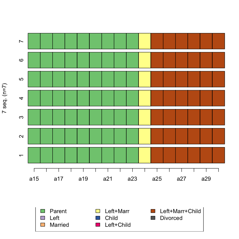
Q2. Plot the pairs of sequences

• Plot the top 5 sequences that are the most similar to sequence 1

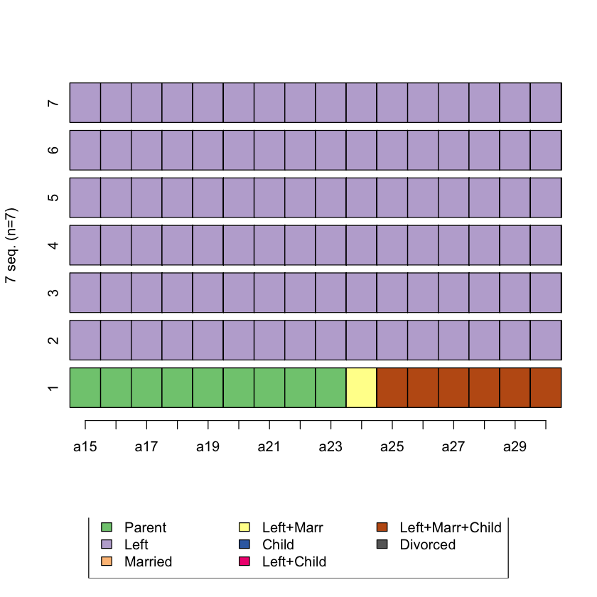
• Plot the top 5 sequences that are the least similar to sequence 1

most_sim <- head(which(biofam.seq.LCS==min(biofam.seq.LCS), arr.ind=T))
most_sim
least_sim <- head(which(biofam.seq.LCS==max(biofam.seq.LCS), arr.ind=T))
least_sim

A matrix: 6 × 2 of type int

	row	col
1167	1	1
1746	39	1
2577	284	1
478	767	1
480	805	1
2380	919	1

A matrix: 6 × 2 of type int

	row	col
2304	443	1
2395	602	1
909	872	1
821	1461	1
769	1546	1
1012	1723	1

# BEGIN SOLUTION
seqiplot(biofam.seq[c(1,most_sim[,1]),])
seqiplot(biofam.seq[c(1,least_sim[,1]),])

# END SOLUTION

Q3. Create a dissimilarity matrix using optimal matching using transition rates as substitution cost matrix

biofam.seq.subcost <- NULL
biofam.seq.OM <- NULL

# BEGIN SOLUTION
biofam.seq.subcost <- seqcost(biofam.seq, method = "TRATE")
biofam.seq.OM <- seqdist(biofam.seq, method='OM', sm=biofam.seq.subcost$sm)
biofam.seq.OM

# END SOLUTION

 [>] creating substitution-cost matrix using transition rates ...

 [>] computing transition probabilities for states Parent/Left/Married/Left+Marr/Child/Left+Child/Left+Marr+Child/Divorced ...

 [>] 2000 sequences with 8 distinct states

 [>] checking 'sm' (size and triangle inequality)

 [>] 537 distinct  sequences 

 [>] min/max sequence lengths: 16/16

 [>] computing distances using the OM metric

 [>] elapsed time: 0.118 secs

A matrix: 2000 × 2000 of type dbl

	1167	514	1013	275	2580	773	1187	47	2091	1846	⋯	278	1980	787	1120	59	629	2297	775	2522	719
1167	0.000000	19.563325	9.890831	21.562411	15.630326	13.901396	13.92295	13.437363	3.957049	19.309299	⋯	13.901396	21.562411	13.878381	11.912527	13.901428	7.636805	17.241790	13.901396	25.83089	7.767166
514	19.563325	0.000000	11.727078	9.916578	7.890831	29.377814	29.50852	13.328194	21.254715	5.777920	⋯	29.377814	9.916578	25.563325	27.388945	29.377846	15.482360	7.695148	29.377814	29.83603	21.414446
1013	9.890831	11.727078	0.000000	11.739494	5.807409	17.661866	17.84715	3.800558	11.559582	15.582221	⋯	17.661866	11.739494	13.836247	15.672997	17.661899	7.755282	9.945416	17.661866	25.89494	13.676236
275	21.562411	9.916578	11.739494	0.000000	5.932086	21.399572	21.78166	11.649872	21.559303	13.954724	⋯	21.399572	0.000000	17.508741	21.431519	21.563325	15.786949	15.643672	21.399572	25.96931	21.719034
2580	15.630326	7.890831	5.807409	5.932086	0.000000	21.529933	21.74830	7.579129	15.627218	9.945416	⋯	21.529933	5.932086	17.672494	19.541064	21.529966	9.854863	9.833155	21.529933	25.93595	15.786949
773	13.901396	29.377814	17.661866	21.399572	21.529933	0.000000	13.89259	19.609357	9.944347	31.430826	⋯	0.000000	21.399572	3.890831	1.988869	5.953968	19.758332	27.500692	0.000000	25.80053	19.888693
1187	13.922955	29.508520	17.847146	21.781663	21.748303	13.892592	0.00000	19.783030	13.913712	31.430901	⋯	13.892592	21.781663	13.923280	13.896816	7.938624	19.758407	27.565217	13.892592	11.90794	19.888768
47	13.437363	13.328194	3.800558	11.649872	7.579129	19.609357	19.78303	0.000000	15.128752	17.183336	⋯	19.609357	11.649872	15.836247	17.620488	19.630873	9.356397	7.945416	19.609357	25.90075	15.288483
2091	3.957049	21.254715	11.559582	21.559303	15.627218	9.944347	13.91371	15.128752	0.000000	21.486480	⋯	9.944347	21.559303	9.921332	7.955477	9.944379	9.813986	19.377592	9.944347	25.82165	9.944347
1846	19.309299	5.777920	15.582221	13.954724	9.945416	31.430826	31.43090	17.183336	21.486480	0.000000	⋯	31.430826	13.954724	27.617910	29.441957	31.430859	11.672494	11.209083	31.430826	31.75841	17.604580
1990	12.771527	26.569874	15.013399	21.168867	20.820808	15.745441	15.89590	13.241680	14.907330	30.083808	⋯	15.745441	21.168867	15.642236	15.577819	15.809924	18.411314	18.874726	15.745441	25.84067	18.382202
2088	13.901396	29.377814	17.661866	21.399572	21.529933	0.000000	13.89259	19.609357	9.944347	31.430826	⋯	0.000000	21.399572	3.890831	1.988869	5.953968	19.758332	27.500692	0.000000	25.80053	19.888693
867	7.781663	11.781663	6.000000	13.780749	7.848663	21.683059	21.70462	7.601116	11.738712	11.527636	⋯	21.683059	13.780749	17.890831	19.694189	21.683091	3.745974	9.491947	21.683059	25.89227	9.678059
1616	7.767166	21.414446	13.676236	21.719034	15.786949	19.888693	19.88877	15.288483	9.944347	17.604580	⋯	19.888693	21.719034	19.865678	17.899824	19.888725	5.932086	18.938618	19.888693	25.84277	0.000000
2136	13.576843	27.206889	15.540463	21.585088	21.237921	15.904540	15.89987	13.878695	15.389537	30.940726	⋯	15.904540	21.585088	15.801335	15.736918	15.875946	19.268232	21.634623	15.904540	25.84465	19.349071
2031	11.957176	21.716753	13.785214	21.854150	15.922778	19.924789	15.94599	15.590790	11.963244	23.644186	⋯	19.924789	21.854150	19.901774	17.935920	15.988880	11.971692	19.761011	19.924789	21.87136	11.953487
2459	13.901396	29.377814	17.661866	21.399572	21.529933	0.000000	13.89259	19.609357	9.944347	31.430826	⋯	0.000000	21.399572	3.890831	1.988869	5.953968	19.758332	27.500692	0.000000	25.80053	19.888693
222	13.901396	29.377814	17.661866	21.399572	21.529933	0.000000	13.89259	19.609357	9.944347	31.430826	⋯	0.000000	21.399572	3.890831	1.988869	5.953968	19.758332	27.500692	0.000000	25.80053	19.888693
2193	11.601116	27.055272	15.328194	21.313058	20.964999	5.904540	13.90765	13.727078	9.379412	30.865892	⋯	5.904540	21.313058	5.801335	5.736918	5.969023	19.193398	21.640674	5.904540	25.81558	19.323759
1571	9.836247	13.836247	10.000000	17.758111	11.826025	23.715382	23.71546	11.601116	13.771035	11.675602	⋯	23.715382	17.758111	19.945416	21.726512	23.715414	4.000000	11.292505	23.715382	25.88537	7.668751
2592	3.789427	21.350553	11.655421	21.655142	15.723056	15.910955	15.91103	15.224591	5.966608	17.540687	⋯	15.910955	21.655142	15.887940	13.922085	15.910987	5.868193	18.874726	15.910955	25.83432	3.977739
1989	9.968180	19.752825	15.916578	23.629412	17.697326	23.825053	23.82513	15.800558	13.880707	17.546903	⋯	23.825053	23.629412	23.802039	21.836184	23.825086	9.810517	15.491947	23.825053	25.85281	3.936360
1917	3.768738	19.451065	9.778571	21.472789	15.540703	15.848887	15.89193	9.890831	5.904540	21.081019	⋯	15.848887	21.472789	15.801335	13.860018	15.848919	9.408525	13.473052	15.848887	25.83670	9.379412
630	17.624605	17.619453	19.732643	25.796257	19.864171	29.746133	29.74621	21.333759	19.801786	13.809587	⋯	29.746133	25.796257	26.000000	27.757263	29.746165	11.977362	17.111679	29.746133	29.74627	9.857439
532	7.767166	21.414446	13.676236	21.719034	15.786949	19.888693	19.88877	15.288483	9.944347	17.604580	⋯	19.888693	21.719034	19.865678	17.899824	19.888725	5.932086	18.938618	19.888693	25.84277	0.000000
863	5.968180	19.643656	11.916578	21.597466	15.665380	19.847315	19.84739	11.800558	9.902968	17.483011	⋯	19.847315	21.597466	19.824300	17.858445	19.847347	5.810517	15.382778	19.847315	25.84436	3.601116
1102	17.537698	13.664729	15.777920	21.841533	15.909447	29.659225	29.65930	17.379035	19.714879	9.854863	⋯	29.659225	21.841533	25.890831	27.670356	29.659257	9.945416	13.156955	29.659225	29.76851	9.770532
1454	13.901396	29.377814	17.661866	21.399572	21.529933	0.000000	13.89259	19.609357	9.944347	31.430826	⋯	0.000000	21.399572	3.890831	1.988869	5.953968	19.758332	27.500692	0.000000	25.80053	19.888693
1174	13.781663	7.836247	3.890831	7.848663	1.916578	21.552698	21.73798	5.662551	15.450414	11.691389	⋯	21.552698	7.848663	17.727078	19.563828	21.552730	9.678059	7.916578	21.552698	25.92563	15.610145
227	9.756035	21.446392	15.665106	21.750980	15.818895	21.877563	21.87764	17.277352	11.933216	17.636526	⋯	21.877563	21.750980	21.854548	19.888693	21.877595	7.920955	18.970564	21.877563	25.84699	1.988869
⋮	⋮	⋮	⋮	⋮	⋮	⋮	⋮	⋮	⋮	⋮	⋱	⋮	⋮	⋮	⋮	⋮	⋮	⋮	⋮	⋮	⋮
81	17.671580	11.945416	7.848663	3.890831	5.977362	17.508741	17.890831	9.727094	17.668472	14.000000	⋯	17.508741	3.890831	13.617910	17.540687	17.672494	13.864171	15.749733	17.508741	25.938624	19.785126
1805	5.838994	21.454157	11.578299	21.578020	15.645934	9.954408	13.924832	15.328194	1.881944	23.368424	⋯	9.954408	21.578020	9.931393	7.965539	9.954440	11.695930	19.577034	9.954408	25.832768	11.826291
789	29.344074	9.826025	19.521157	7.781663	13.713748	29.181235	29.563325	19.431535	29.340966	13.864171	⋯	29.181235	7.781663	25.290404	29.213181	29.344988	23.568611	17.521173	29.181235	29.890831	29.500697
2361	17.892267	29.617689	17.956315	21.890831	21.857472	17.861904	3.969312	19.892199	17.883024	31.540070	⋯	17.861904	21.890831	17.892592	17.866128	11.907936	19.867576	27.641296	17.861904	7.938624	19.888790
56	1.968180	19.534487	9.861993	21.533573	15.601488	15.869576	15.891135	11.691389	5.925230	19.280461	⋯	15.869576	21.533573	15.833155	13.880707	15.869608	7.607967	15.273610	15.869576	25.835909	7.578854
645	5.691389	17.427776	7.732643	17.732364	11.800279	17.812917	17.812992	11.301813	7.868570	13.617910	⋯	17.812917	17.732364	14.000000	15.824047	17.812949	1.945416	15.183336	17.812917	25.860785	5.943593
1721	5.800558	17.363883	5.807409	17.546903	11.614818	13.793800	13.945989	7.636805	7.491947	21.219025	⋯	13.793800	17.546903	10.000000	11.804930	13.793832	9.546531	13.781663	13.793800	25.853925	13.522447
1419	13.901418	29.377836	17.661888	21.508741	21.529955	3.969312	9.923280	19.609379	9.944368	31.430848	⋯	3.969312	21.508741	4.000000	3.973536	1.984656	19.758354	27.500713	3.969312	21.831216	19.888715
1207	21.562411	9.916578	11.739494	0.000000	5.932086	21.399572	21.781663	11.649872	21.559303	13.954724	⋯	21.399572	0.000000	17.508741	21.431519	21.563325	15.786949	15.643672	21.399572	25.969312	21.719034
259	13.922955	29.508520	17.847146	21.781663	21.748303	13.892592	0.000000	19.783030	13.913712	31.430901	⋯	13.892592	21.781663	13.923280	13.896816	7.938624	19.758407	27.565217	13.892592	11.907936	19.888768
2413	13.663439	9.778571	10.000000	17.681818	11.749733	27.564835	27.586393	8.000000	17.620488	9.524544	⋯	27.564835	17.681818	23.836247	25.575965	27.564867	9.691389	3.800558	27.564835	27.847719	15.160698
2090	21.562411	9.916578	11.739494	0.000000	5.932086	21.399572	21.781663	11.649872	21.559303	13.954724	⋯	21.399572	0.000000	17.508741	21.431519	21.563325	15.786949	15.643672	21.399572	25.969312	21.719034
1337	1.800558	19.479903	9.807409	21.501627	15.569541	13.880707	13.923749	11.636805	3.936360	21.109857	⋯	13.880707	21.501627	13.833155	11.891838	13.880739	9.437363	15.441232	13.880707	25.831685	9.567724
1826	7.859011	15.698240	9.916578	17.674688	11.742602	21.749277	21.749352	9.800558	11.804930	13.560233	⋯	21.749277	17.674688	18.000000	19.760407	21.749309	3.916578	11.437363	21.749277	25.870821	7.523893
2503	11.002789	26.627550	15.071076	21.226544	20.878485	11.809081	13.922702	13.299356	10.970970	30.300958	⋯	11.809081	21.226544	11.705875	11.641458	11.873563	18.628464	19.273610	11.809081	25.830638	18.758825
106	1.800558	21.318607	11.623475	21.623196	15.691110	13.922085	13.922160	15.192644	3.977739	17.508741	⋯	13.922085	21.623196	13.899070	11.933216	13.922117	5.836247	19.042348	13.922085	25.830097	5.966608
1181	12.000000	15.781663	6.000000	9.698240	9.691389	13.640674	13.989674	7.916578	13.600837	19.636805	⋯	13.640674	9.698240	9.781663	13.473052	13.771337	13.732643	14.000000	13.640674	25.897610	19.631337
1848	12.771527	26.569874	15.013399	21.168867	20.820808	15.745441	15.895901	13.241680	14.907330	30.083808	⋯	15.745441	21.168867	15.642236	15.577819	15.809924	18.411314	18.874726	15.745441	25.840675	18.382202
2203	19.616996	10.000000	9.794079	1.945416	5.954724	19.454157	19.836247	9.704456	19.613888	13.977362	⋯	19.454157	1.945416	15.563325	19.486103	19.617910	13.841533	15.666310	19.454157	25.953968	19.773619
1745	21.434627	1.916578	13.473052	8.000000	7.836247	29.355050	29.518846	15.244772	21.431519	5.954724	⋯	29.355050	8.000000	25.508741	27.366180	29.355082	15.659164	9.611726	29.355050	29.846352	21.591249
278	13.901396	29.377814	17.661866	21.399572	21.529933	0.000000	13.892592	19.609357	9.944347	31.430826	⋯	0.000000	21.399572	3.890831	1.988869	5.953968	19.758332	27.500692	0.000000	25.800528	19.888693
1980	21.562411	9.916578	11.739494	0.000000	5.932086	21.399572	21.781663	11.649872	21.559303	13.954724	⋯	21.399572	0.000000	17.508741	21.431519	21.563325	15.786949	15.643672	21.399572	25.969312	21.719034
787	13.878381	25.563325	13.836247	17.508741	17.672494	3.890831	13.923280	15.836247	9.921332	27.617910	⋯	3.890831	17.508741	0.000000	3.922778	5.984656	15.945416	23.781663	3.890831	25.831216	19.865678
1120	11.912527	27.388945	15.672997	21.431519	19.541064	1.988869	13.896816	17.620488	7.955477	29.441957	⋯	1.988869	21.431519	3.922778	0.000000	5.958192	17.769463	25.511822	1.988869	25.804752	17.899824
59	13.901428	29.377846	17.661899	21.563325	21.529966	5.953968	7.938624	19.630873	9.944379	31.430859	⋯	5.953968	21.563325	5.984656	5.958192	0.000000	19.758365	27.500724	5.953968	19.846560	19.888725
629	7.636805	15.482360	7.755282	15.786949	9.854863	19.758332	19.758407	9.356397	9.813986	11.672494	⋯	19.758332	15.786949	15.945416	17.769463	19.758365	0.000000	13.237921	19.758332	25.876128	5.932086
2297	17.241790	7.695148	9.945416	15.643672	9.833155	27.500692	27.565217	7.945416	19.377592	11.209083	⋯	27.500692	15.643672	23.781663	25.511822	27.500724	13.237921	0.000000	27.500692	27.859633	18.938618
775	13.901396	29.377814	17.661866	21.399572	21.529933	0.000000	13.892592	19.609357	9.944347	31.430826	⋯	0.000000	21.399572	3.890831	1.988869	5.953968	19.758332	27.500692	0.000000	25.800528	19.888693
2522	25.830891	29.836026	25.894939	25.969312	25.935952	25.800528	11.907936	25.900751	25.821648	31.758407	⋯	25.800528	25.969312	25.831216	25.804752	19.846560	25.876128	27.859633	25.800528	0.000000	25.842769
719	7.767166	21.414446	13.676236	21.719034	15.786949	19.888693	19.888768	15.288483	9.944347	17.604580	⋯	19.888693	21.719034	19.865678	17.899824	19.888725	5.932086	18.938618	19.888693	25.842769	0.000000

?seqdist

Q4. Perform an agglomerative clustering using ward linkage method

• You should use the dissimilarity matrix with optimal matching generated in Q3

• Plot the dendogram

clusterward <- NULL

# BEGIN SOLUTION

clusterward <- agnes(biofam.seq.OM, diss = TRUE, method = "ward")

# Run this to generate the dendogram
plot(clusterward, which.plot=2)

# END SOLUTION

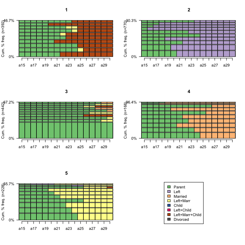
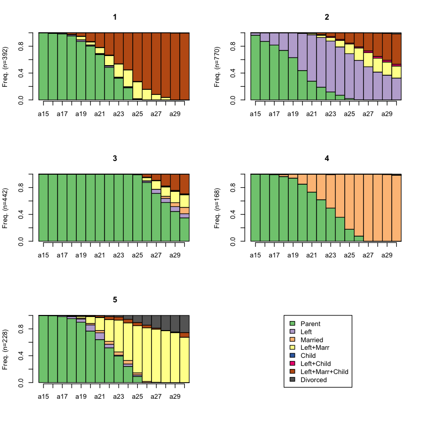
Q5: Select clusters

• Cut the dendogram tree as appropriate using the cutree() function

• List the number of observations in each cluster

• Plot the sequence frequency by cluster membership (hint: seqfplot())

• Plot the state distribution by cluster membership (hint: seqdplot())

# BEGIN SOLUTION

# cut the dendogram tree to generate two clusters
cluster5 <- cutree(clusterward, k = 5)

# check the number of observations in each cluster
table(cluster5)

# plot sequence frequency by cluster membership
seqfplot(biofam.seq, group = cluster5, pbarw = T)

# plot state distribution by cluster membership
seqdplot(biofam.seq, group = cluster5)

# END SOLUTION


s1 = Read (2) - Write (2)
s2 = Read(5) - Write (5)

cluster5
  1   2   3   4   5 
392 770 442 168 228 

Error in Read(2): could not find function "Read"
Traceback:

?seqcost()

seqcost {TraMineR}

R Documentation

Generate substitution and indel costs

Description

The function seqcost proposes different ways to generate substitution costs (supposed to represent state dissimilarities) and possibly indel costs. Proposed methods are: "CONSTANT" (same cost for all substitutions), "TRATE" (derived from the observed transition rates), "FUTURE" (Chi-squared distance between conditional state distributions lag positions ahead), "FEATURES" (Gower distance between state features), "INDELS", "INDELSLOG" (based on estimated indel costs). The substitution-cost matrix is intended to serve as sm argument in the seqdist function that computes distances between sequences. seqsubm is an alias that returns only the substitution cost matrix, i.e., no indel.

Usage

seqcost(seqdata, method, cval = NULL, with.missing = FALSE, miss.cost = NULL,
  time.varying = FALSE, weighted = TRUE, transition = "both", lag = 1,
  miss.cost.fixed = NULL, state.features = NULL, feature.weights = NULL,
  feature.type = list(), proximities = FALSE)

seqsubm(...)

Arguments

seqdata	A sequence object as returned by the seqdef function.
method	String. How to generate the costs. One of "CONSTANT" (same cost for all substitutions), "TRATE" (derived from the observed transition rates), "FUTURE" (Chi-squared distance between conditional state distributions lag positions ahead), "FEATURES" (Gower distance between state features), "INDELS", "INDELSLOG" (based on estimated indel costs).
cval	Scalar. For method "CONSTANT", the single substitution cost. For method "TRATE", a base value from which transition probabilities are subtracted. If NULL, cval=2 is used, unless transition is "both" and time.varying is TRUE, in which case cval=4.
with.missing	Logical. Should an additional entry be added in the matrix for the missing states? If TRUE, the ‘missing’ state is also added to the alphabet. Set as TRUE if you want to use the costs for distances between sequences containing non deleted (non void) missing values. Forced as FALSE when there are no non-void missing values in seqdata. See Gabadinho et al. (2010) for more details on the options for handling missing values when creating the state sequence object with seqdef.
miss.cost	Scalar or vector. Cost for substituting the missing state. Default is cval.
miss.cost.fixed	Logical. Should the substitution cost for missing be set as the miss.cost value. When NULL (default) it will be set as FALSE when method = "INDELS" or "INDELSLOG", and TRUE otherwise.
time.varying	Logical. If TRUE return an array with a distinct matrix for each time unit. Time is the third dimension (subscript) of the returned array. Time varying works only with method='CONSTANT', 'TRATE', 'INDELS', and 'INDELSLOG'.
weighted	Logical. Should weights in seqdata be used when applicable?
transition	String. Only used if method="TRATE" and time.varying=TRUE. On which transition are rates based? Should be one of "previous" (from previous state), "next" (to next state) or "both".
lag	Integer. For methods TRATE and FUTURE only. Time ahead to which transition rates are computed (default is lag=1).
state.features	Data frame with features values for each state.
feature.weights	Vector of feature weights with length equal to the number of columns of state.features.
feature.type	List of feature types. See daisy for details.
proximities	Logical: should state proximities be returned instead of substitution costs?
...	Arguments passed to seqcost

Details

The substitution-cost matrix has dimension ns*ns, where ns is the number of states in the alphabet of the sequence object. The element (i,j) of the matrix is the cost of substituting state i with state j. It represents the dissimilarity between the states i and j. The indel cost of the cost of inserting or deleting a state.

With method CONSTANT, the substitution costs are all set equal to the cval value, the default value being 2.

With method TRATE (transition rates), the transition probabilities between all pairs of states is first computed (using the seqtrate function). Then, the substitution cost between states i and j is obtained with the formula

SC(i,j) = cval - P(i|j) -P(j|i)

where P(i|j) is the probability of transition from state j to i lag positions ahead. Default cval value is 2. When time.varying=TRUE and transition="both", the substitution cost at position t is set as

SC(i,j,t) = cval - P(i|j,t-1) -P(j|i,t-1) - P(i|j,t) - P(j|i,t)

where P(i|j,t-1) is the probability to transit from state j at t-1 to i at t. Here, the default cval value is 4.

With method FUTURE, the cost between i and j is the Chi-squared distance between the vector (d(alphabet | i)) of probabilities of transition from states i and j to all the states in the alphabet lag positions ahead:

SC(i,j) = ChiDist(d(alphabet | i), d(alphabet | j))

With method FEATURES, each state is characterized by the variables state.features, and the cost between i and j is computed as the Gower distance between their vectors of state.features values.

With methods INDELS and INDELSLOG, values of indels are first derived from the state relative frequencies f_i. For INDELS, indel_i = 1/f_i is used, and for INDELSLOG, indel_i = log[2/(1 + f_i)]. Substitution costs are then set as SC(i,j) = indel_i + indel_j.

For all methods but INDELS and INDELSLOG, the indel is set as max(sm)/2 when time.varying=FALSE and as 1 otherwise.

Value

For seqcost, a list of two elements, indel and sm or prox:

indel	The indel cost. Either a scalar or a vector of size ns. When time.varying=TRUE and method is one of "INDELS" or "INDELSLOG", a matrix with indels per time point in columns.
sm	The substitution-cost matrix (or array) when proximities = FALSE (default).
prox	The state proximity matrix when proximities = TRUE.

sm and prox are, when time.varying = FALSE, a matrix of size ns * ns, where ns is the number of states in the alphabet of the sequence object. When time.varying = TRUE, they are a three dimensional array of size ns * ns * L, where L is the maximum sequence length.

For seqsubm, only one element, the matrix (or array) sm.

Author(s)

Gilbert Ritschard and Matthias Studer (and Alexis Gabadinho for first version of seqsubm)

References

Gabadinho, A., G. Ritschard, N. S. Müller and M. Studer (2011). Analyzing and Visualizing State Sequences in R with TraMineR. Journal of Statistical Software 40(4), 1-37.

Gabadinho, A., G. Ritschard, M. Studer and N. S. Müller (2010). Mining Sequence Data in R with the TraMineR package: A user's guide. Department of Econometrics and Laboratory of Demography, University of Geneva.

Studer, M. & Ritschard, G. (2016), "What matters in differences between life trajectories: A comparative review of sequence dissimilarity measures", Journal of the Royal Statistical Society, Series A. 179(2), 481-511. doi: 10.1111/rssa.12125

Studer, M. and G. Ritschard (2014). "A Comparative Review of Sequence Dissimilarity Measures". LIVES Working Papers, 33. NCCR LIVES, Switzerland, 2014. doi: 10.12682/lives.2296-1658.2014.33

See Also

seqtrate, seqdef, seqdist.

Examples

## Defining a sequence object with columns 10 to 25
## of a subset of the 'biofam' example data set.
data(biofam)
biofam.seq <- seqdef(biofam[501:600,10:25])

## Indel and substitution costs based on log of inverse state frequencies
lifcost <- seqcost(biofam.seq, method="INDELSLOG")
## Here lifcost$indel is a vector
biofam.om <- seqdist(biofam.seq, method="OM", indel=lifcost$indel, sm=lifcost$sm)

## Optimal matching using transition rates based substitution-cost matrix
## and the associated indel cost
## Here trcost$indel is a scalar
trcost <- seqcost(biofam.seq, method="TRATE")
biofam.om <- seqdist(biofam.seq, method="OM", indel=trcost$indel, sm=trcost$sm)

## Using costs based on FUTURE with a forward lag of 4
fucost <- seqcost(biofam.seq, method="FUTURE", lag=4)
biofam.om <- seqdist(biofam.seq, method="OM", indel=fucost$indel, sm=fucost$sm)

## Optimal matching using a unique substitution cost of 2
## and an insertion/deletion cost of 3
ccost <- seqsubm(biofam.seq, method="CONSTANT", cval=2)
biofam.om.c2 <- seqdist(biofam.seq, method="OM",indel=3, sm=ccost)

## Displaying the distance matrix for the first 10 sequences
biofam.om.c2[1:10,1:10]

## =================================
## Example with weights and missings
## =================================
data(ex1)
ex1.seq <- seqdef(ex1[,1:13], weights=ex1$weights)

## Unweighted
subm <- seqcost(ex1.seq, method="INDELSLOG", with.missing=TRUE, weighted=FALSE)
ex1.om <- seqdist(ex1.seq, method="OM", indel=subm$indel, sm=subm$sm, with.missing=TRUE)

## Weighted
subm.w <- seqcost(ex1.seq, method="INDELSLOG", with.missing=TRUE, weighted=TRUE)
ex1.omw <- seqdist(ex1.seq, method="OM", indel=subm.w$indel, sm=subm.w$sm, with.missing=TRUE)

ex1.om == ex1.omw

---

[Package TraMineR version 2.2-3 ]

previous

Lab 1: Exploratory analysis of sequential data in education

next

Lab 3