![]()
Lecture 1: Exploratory data analysis of sequence data in education
Quan Nguyen, Department of Statistics, University of British Columbia
Learning objectives:
By the end of this lecture, workshop participants should be able to:
Understand the type of questions that are relevant to clustering of sequential data
Understand different types of sequence data format and convert between formats
Create a sequence object from an existing dataset using the
TraMineRpackageManipulate sequence object to deal with missing values and misaligned sequences
Visualize and compute descriptive statitsics to explore sequential data
1. Why do we want to perform cluster analysis on sequential data in education?
What types of temporal/sequential data exist in education?
Data source |
Time granularity |
Questions |
|---|---|---|
SIS records |
Semester/Year |
What are the common study paths taken by students based on their course enrolment? |
LMS log files |
Seconds/Daily/Semester |
What are the common learning patterns of students during a course? |
Eye-tracking |
Miliseconds/Seconds/Minutes |
What are the common thought process when students engage in an exercise? |
Videos |
Frames/Seconds/Minutes |
What are the common interaction patterns of students during collaborative activities? |
What type of research questions that are temporal/sequential specific?
Exploratory: What are the common patterns exist in the data?
Predictive: Can we classifiy an existing sequence? Can we predict the next activity/outcome given a sequence?
Causal: Does X cause Y?
Introduction to the TramineR package
TraMineR is a R-package for mining, describing and visualizing sequences of states or events, and more generally discrete sequence data
Some common usage of TramineR includes:
Visualize sequences
Explore sequences with descriptive statistics (e.g., frequencies, transitional probabilities, entropy)
Cluster analysis of sequences (e.g., Optimal matching/Edit distances)
Run discrepancy analyses to study how sequences are related to covariates
Installation in R:
install.packages("TraMineR", dependencies=TRUE)
# install.packages("TraMineR")
options(repr.plot.width=15, repr.plot.height=8)
library("TraMineR")
packageVersion("TraMineR")
library(readr)
library(tidyverse)
Warning message:
“package ‘TraMineR’ was built under R version 4.1.1”
TraMineR stable version 2.2-3 (Built: 2022-01-26)
Website: http://traminer.unige.ch
Please type 'citation("TraMineR")' for citation information.
[1] ‘2.2.3’
Warning message:
“package ‘readr’ was built under R version 4.1.1”
── Attaching packages ──────────────────────────────────────────────────────────────────────────── tidyverse 1.3.1 ──
✔ ggplot2 3.3.5     ✔ dplyr   1.0.7
✔ tibble  3.1.5     ✔ stringr 1.4.0
✔ tidyr   1.1.3     ✔ forcats 0.5.1
✔ purrr   0.3.4
Warning message:
“package ‘tibble’ was built under R version 4.1.1”
── Conflicts ─────────────────────────────────────────────────────────────────────────────── tidyverse_conflicts() ──
✖ dplyr::filter() masks stats::filter()
✖ dplyr::lag()    masks stats::lag()
Some terminologies
States vs events
States: Read, write, discuss, review
Events: Read -> Write, Write -> Discuss (each change of state is an event)
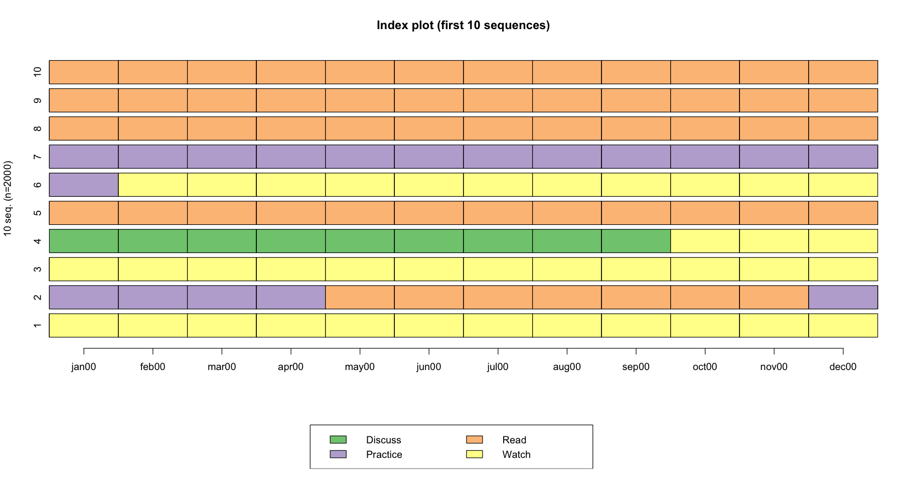
As see in the example below, the sequences 7,8,9,10 no event occurred during the observation period since the respondent stays in the same state during the whole sequence
In sequence 2, two events occurred: Practice -> Read, and Read -> Practice
data(actcal)
actcal <- data.frame(lapply(actcal, function(x) { gsub("^A\\b", "Read", x)}))
actcal <- data.frame(lapply(actcal, function(x) { gsub("^B\\b", "Watch", x)}))
actcal <- data.frame(lapply(actcal, function(x) { gsub("^C\\b", "Discuss", x)}))
actcal <- data.frame(lapply(actcal, function(x) { gsub("^D\\b", "Practice", x)}))
actcal.seq <- seqdef(actcal, var = 13:24)
# actcal.seq
seqiplot(actcal.seq, main = "Index plot (first 10 sequences)",with.legend = TRUE)
[>] 4 distinct states appear in the data:
1 = Discuss
2 = Practice
3 = Read
4 = Watch
[>] state coding:
[alphabet] [label] [long label]
1 Discuss Discuss Discuss
2 Practice Practice Practice
3 Read Read Read
4 Watch Watch Watch
[>] 2000 sequences in the data set
[>] min/max sequence length: 12/12
The alphabet is the number of unique states (or events) in the data. In the example above, we have four unique states (i.e., Read, Discuss, Practice, Watch) so the alphabet = 4
alphabet(actcal.seq)
- 'Discuss'
- 'Practice'
- 'Read'
- 'Watch'
Time reference: Internal and external clocks
Internal: Year 1, Year 2, Year 3 or Semester 1, Semester 2, Semester 3
External: June 17th, 2022, or 14:30:00 PST
2. Data manipulation with sequences
Data format
The ‘states-sequence’ (STS) format
Each row is an individual
In this format, the successive states (statuses) of an individual are given in consecutive columns. Each column is supposed to correspond to a predetermined time unit
head(actcal.seq)
| jan00 | feb00 | mar00 | apr00 | may00 | jun00 | jul00 | aug00 | sep00 | oct00 | nov00 | dec00 | |
|---|---|---|---|---|---|---|---|---|---|---|---|---|
| <fct> | <fct> | <fct> | <fct> | <fct> | <fct> | <fct> | <fct> | <fct> | <fct> | <fct> | <fct> | |
| 1 | Watch | Watch | Watch | Watch | Watch | Watch | Watch | Watch | Watch | Watch | Watch | Watch |
| 2 | Practice | Practice | Practice | Practice | Read | Read | Read | Read | Read | Read | Read | Practice |
| 3 | Watch | Watch | Watch | Watch | Watch | Watch | Watch | Watch | Watch | Watch | Watch | Watch |
| 4 | Discuss | Discuss | Discuss | Discuss | Discuss | Discuss | Discuss | Discuss | Discuss | Watch | Watch | Watch |
| 5 | Read | Read | Read | Read | Read | Read | Read | Read | Read | Read | Read | Read |
| 6 | Practice | Watch | Watch | Watch | Watch | Watch | Watch | Watch | Watch | Watch | Watch | Watch |
The ‘state-permanence-sequence’ (SPS) format
Each row is an individual
Each successive distinct state in the sequence is given together with its duration
# print(head(actcal.seq), format='SPS')
actcal.sps <- seqformat(actcal, 13:24, from = "STS", to = "SPS", compress = TRUE)
head(actcal.sps)
[>] converting STS sequences to 2000 SPS sequences
[>] compressing SPS sequences
| Sequence | |
|---|---|
| 1 | (Watch,12) |
| 2 | (Practice,4)-(Read,7)-(Practice,1) |
| 3 | (Watch,12) |
| 4 | (Discuss,9)-(Watch,3) |
| 5 | (Read,12) |
| 6 | (Practice,1)-(Watch,11) |
The vertical ‘time-stamped-event’ (TSE) format
Each row is an event
Each record of the TSE representation usually contains a case identifier, a time stamp and codes identifying the event occurring
tstate <- seqetm(actcal.seq, method='state')
actcal.tse <- seqformat(actcal, 13:24, from = "STS", to = "TSE", tevent=tstate)
head(actcal.tse)
[!!] 'id' set to NULL as it is not specified (backward compatibility with TraMineR 1.8)
[!!] replacing original IDs in the output by the sequence indexes
[>] converting STS sequences to 2579 TSE sequences
| id | time | event | |
|---|---|---|---|
| <dbl> | <dbl> | <chr> | |
| 1 | 1 | 0 | Watch |
| 2 | 2 | 0 | Practice |
| 3 | 2 | 4 | Read |
| 4 | 2 | 11 | Practice |
| 5 | 3 | 0 | Watch |
| 6 | 4 | 0 | Discuss |
The spell (SPELL) format
Each row is a state
Each record of SPELL contains an ID, start time, end time, and the state
actcal.spell <- seqformat(actcal, 13:24, from = "STS", to = "SPELL")
head(actcal.seq)
head(actcal.spell)
[>] converting STS sequences to 2579 spells
| jan00 | feb00 | mar00 | apr00 | may00 | jun00 | jul00 | aug00 | sep00 | oct00 | nov00 | dec00 | |
|---|---|---|---|---|---|---|---|---|---|---|---|---|
| <fct> | <fct> | <fct> | <fct> | <fct> | <fct> | <fct> | <fct> | <fct> | <fct> | <fct> | <fct> | |
| 1 | Watch | Watch | Watch | Watch | Watch | Watch | Watch | Watch | Watch | Watch | Watch | Watch |
| 2 | Practice | Practice | Practice | Practice | Read | Read | Read | Read | Read | Read | Read | Practice |
| 3 | Watch | Watch | Watch | Watch | Watch | Watch | Watch | Watch | Watch | Watch | Watch | Watch |
| 4 | Discuss | Discuss | Discuss | Discuss | Discuss | Discuss | Discuss | Discuss | Discuss | Watch | Watch | Watch |
| 5 | Read | Read | Read | Read | Read | Read | Read | Read | Read | Read | Read | Read |
| 6 | Practice | Watch | Watch | Watch | Watch | Watch | Watch | Watch | Watch | Watch | Watch | Watch |
| id | begin | end | states | |
|---|---|---|---|---|
| <chr> | <dbl> | <dbl> | <fct> | |
| 1 | 1 | 1 | 12 | Watch |
| 2 | 2 | 1 | 4 | Practice |
| 3 | 2 | 5 | 11 | Read |
| 4 | 2 | 12 | 12 | Practice |
| 5 | 3 | 1 | 12 | Watch |
| 6 | 4 | 1 | 9 | Discuss |
Converting between format
seqformat(data, var = ..., from = "...", to = ",,,", compress = FALSE/TRUE)
Examples:
seqformat(actcal, 13:24, from = "STS", to = "SPELL")seqformat(actcal, 13:24, from = "STS", to = "SPS", compress = TRUE)
Create a sequence object from data
We can use the seqdef function to create a sequence object from an existing dataframe.
In the dataset actcal below, it consists of:
The sequence data were collected on a monthly basis on each participant in columns: “jan00”, “feb00”, “mar00”, “apr00”, “may00”, “jun00”, “jul00”, “aug00”, “sep00”, “oct00”, “nov00”, “dec00”
The covariates such as age, education, region, etc…
head(actcal)
| idhous00 | age00 | educat00 | civsta00 | nbadul00 | nbkid00 | aoldki00 | ayouki00 | region00 | com2.00 | ⋯ | mar00 | apr00 | may00 | jun00 | jul00 | aug00 | sep00 | oct00 | nov00 | dec00 | |
|---|---|---|---|---|---|---|---|---|---|---|---|---|---|---|---|---|---|---|---|---|---|
| <chr> | <chr> | <chr> | <chr> | <chr> | <chr> | <chr> | <chr> | <chr> | <chr> | ⋯ | <chr> | <chr> | <chr> | <chr> | <chr> | <chr> | <chr> | <chr> | <chr> | <chr> | |
| 1 | 60671 | 47 | maturity | married | 3 | 2 | 17 | 14 | Middleland (BE, FR, SO, NE, JU) | Industrial and tertiary sector communes | ⋯ | Watch | Watch | Watch | Watch | Watch | Watch | Watch | Watch | Watch | Watch |
| 2 | 25321 | 21 | maturity | single, never married | 2 | 0 | -3 | -3 | Zurich | Suburban communes | ⋯ | Practice | Practice | Read | Read | Read | Read | Read | Read | Read | Practice |
| 3 | 53221 | 50 | full-time vocational school | married | 2 | 0 | -3 | -3 | Lake Geneva (VD, VS, GE) | Peripheral urban communes | ⋯ | Watch | Watch | Watch | Watch | Watch | Watch | Watch | Watch | Watch | Watch |
| 4 | 13911 | 37 | maturity | single, never married | 1 | 0 | -3 | -3 | Middleland (BE, FR, SO, NE, JU) | Centres | ⋯ | Discuss | Discuss | Discuss | Discuss | Discuss | Discuss | Discuss | Watch | Watch | Watch |
| 5 | 145301 | 20 | apprenticeship | single, never married | 3 | 0 | -3 | -3 | North-west Switzerland (BS, BL, AG) | Rural commuter communes | ⋯ | Read | Read | Read | Read | Read | Read | Read | Read | Read | Read |
| 6 | 40022 | 27 | university, higher specialized school | single, never married | 2 | 0 | -3 | -3 | Central Switzerland (LU, UR, SZ, OW, NW, ZG) | Suburban communes | ⋯ | Watch | Watch | Watch | Watch | Watch | Watch | Watch | Watch | Watch | Watch |
To create the sequence, we can use the seqdef() function.
We can see that there were 2000 sequences, with the length of 12, and consists of 4 states
actcal.seq <- seqdef(actcal, var = c("jan00", "feb00", "mar00",
         "apr00", "may00", "jun00", "jul00", "aug00", "sep00", "oct00",
         "nov00", "dec00"))
[>] 4 distinct states appear in the data:
1 = Discuss
2 = Practice
3 = Read
4 = Watch
[>] state coding:
[alphabet] [label] [long label]
1 Discuss Discuss Discuss
2 Practice Practice Practice
3 Read Read Read
4 Watch Watch Watch
[>] 2000 sequences in the data set
[>] min/max sequence length: 12/12
But this is a relatively clean data set, because it has defined a time unit (monthly). There were also no missing value or no misalignment in the timing of data collection (everyone started and ended at the same time).
Import a log file
Let’s try to process a more messy example of a log file lasi21_logdata.csv. The dataset consists of 852,458 records and 9 columns
idrefers to anonymized student IDsas_id_siterefers to the id of the site that students visitedsite_typerefers to the type of content (e.g., resource, homepage, forumng, …)date_timereferes to the timestampspent_timerefers to the estimated dwell time in milisecondsactionrefers to the type of action took place (e.g., view, download, etc..)instancenamerefers to the type of content (e.g., chapter 1, chapter 2, assignment 1, etc..)avg scorerefers to the final scorePassFlagrefers to a binary class of whether students passed or failed the course
lasi21_logdata <- read_csv("~/Downloads/lasi21_logdata.csv")
head(lasi21_logdata)
Rows: 852458 Columns: 9
── Column specification ─────────────────────────────────────────────────────────────────────────────────────────────
Delimiter: ","
chr  (3): site_type, action, instancename
dbl  (5): id, sas_id_site, spent_time, avg score, PassFlag
dttm (1): date_time
ℹ Use `spec()` to retrieve the full column specification for this data.
ℹ Specify the column types or set `show_col_types = FALSE` to quiet this message.
| id | sas_id_site | site_type | date_time | spent_time | action | instancename | avg score | PassFlag |
|---|---|---|---|---|---|---|---|---|
| <dbl> | <dbl> | <chr> | <dttm> | <dbl> | <chr> | <chr> | <dbl> | <dbl> |
| 1 | 872750 | content | 2017-01-22 02:16:00 | 1000 | apiset | Block 2 Part 2 | 26 | 0 |
| 1 | 872771 | content | 2017-02-15 14:47:00 | 12000 | view | Block 3 Part 7 | 26 | 0 |
| 1 | 872750 | content | 2017-01-22 01:58:00 | 1000 | apiset | Block 2 Part 2 | 26 | 0 |
| 1 | 872750 | content | 2017-01-22 02:16:00 | 1000 | apiset | Block 2 Part 2 | 26 | 0 |
| 1 | 872890 | studio | 2016-12-01 20:23:00 | 58000 | view work stream (1) | studio | 26 | 0 |
| 1 | 872859 | forumng | 2017-03-14 14:59:00 | 2000 | view discussion | forumng | 26 | 0 |
# Fixing some typos
lasi21_logdata$site_type <- ifelse(grepl("ssignment", lasi21_logdata$instancename), "assignment",lasi21_logdata$site_type )
lasi21_logdata$site_type <- ifelse(grepl("exam", lasi21_logdata$instancename), "assignment",lasi21_logdata$site_type )

# Convert dataframe to data.table for faster processing
lasi21_logdata <- lasi21_logdata %>% select(id,date_time,spent_time,site_type)

head(lasi21_logdata)
| id | date_time | spent_time | site_type |
|---|---|---|---|
| <dbl> | <dttm> | <dbl> | <chr> |
| 1 | 2017-01-22 02:16:00 | 1000 | content |
| 1 | 2017-02-15 14:47:00 | 12000 | content |
| 1 | 2017-01-22 01:58:00 | 1000 | content |
| 1 | 2017-01-22 02:16:00 | 1000 | content |
| 1 | 2016-12-01 20:23:00 | 58000 | studio |
| 1 | 2017-03-14 14:59:00 | 2000 | forumng |
Now we need to make some decisions:
What is a sequence in our data? (i.e., what each row will represent)
Each sequence could be a student
Each sequence could be a learning session (defined as consecutive learning activities of at least 60s with no more than 30 minutes break between activities)
What is the time unit in our data?
Every minute?
Every 5 mins?
Every hour?
# convert ms to minutes
lasi21_logdata$spent_time_m <- round(lasi21_logdata$spent_time/60000, digits=1)

# create a flag for session break (aka where time spent > 30 minutes)
lasi21_logdata$session_flag <- 0
lasi21_logdata$session_flag <- ifelse(lasi21_logdata$spent_time_m>30, 1, lasi21_logdata$session_flag)

# filter out all spent_time < 90s
lasi21_logdata2 <- lasi21_logdata %>%  filter(spent_time>=90000)


# create session number
lasi21_logdata2 <- lasi21_logdata2 %>%
                        arrange(id,date_time,spent_time) %>%
                        mutate(session_num = cumsum(session_flag))

# remove session break
lasi21_logdata2 <- lasi21_logdata2 %>%  filter(session_flag==0)

# for each learning session, calculate the cummulative time spent
lasi21_logdata2 <- lasi21_logdata2 %>%
                        arrange(id,date_time,spent_time) %>%
                        group_by(session_num) %>%
                        mutate(spent_time_m_cum = cumsum(spent_time_m))

# create time unit as 1 minute (60s)
lasi21_logdata2$time_unit <- round(lasi21_logdata2$spent_time_m_cum,digits=0)
head(lasi21_logdata2,10)
| id | date_time | spent_time | site_type | spent_time_m | session_flag | session_num | spent_time_m_cum | time_unit |
|---|---|---|---|---|---|---|---|---|
| <dbl> | <dttm> | <dbl> | <chr> | <dbl> | <dbl> | <dbl> | <dbl> | <dbl> |
| 1 | 2016-09-06 18:19:00 | 217000 | content | 3.6 | 0 | 1 | 3.6 | 4 |
| 1 | 2016-09-06 18:22:00 | 397000 | content | 6.6 | 0 | 1 | 10.2 | 10 |
| 1 | 2016-09-06 18:29:00 | 337000 | content | 5.6 | 0 | 1 | 15.8 | 16 |
| 1 | 2016-09-06 18:34:00 | 182000 | content | 3.0 | 0 | 1 | 18.8 | 19 |
| 1 | 2016-09-06 18:38:00 | 178000 | content | 3.0 | 0 | 1 | 21.8 | 22 |
| 1 | 2016-09-07 13:43:00 | 323000 | content | 5.4 | 0 | 3 | 5.4 | 5 |
| 1 | 2016-09-07 13:48:00 | 1298000 | content | 21.6 | 0 | 3 | 27.0 | 27 |
| 1 | 2016-09-07 14:10:00 | 1576000 | content | 26.3 | 0 | 3 | 53.3 | 53 |
| 1 | 2016-09-07 18:16:00 | 522000 | content | 8.7 | 0 | 4 | 8.7 | 9 |
| 1 | 2016-09-07 18:24:00 | 91000 | content | 1.5 | 0 | 4 | 10.2 | 10 |
Prepare data in SPELL format
Since the log data can capture the start time and end time of each visit, it makes it suitable to prepare the data in a SPELL format.
To recall, the structure of a SPELL data format should look like this
Position |
Varible |
Option name |
|---|---|---|
1 |
ID |
id |
2 |
Start time |
begin |
3 |
End time |
end |
4 |
Status |
status |
log_spell <- lasi21_logdata2 %>%
            group_by(session_num) %>%
            mutate(start = lag(time_unit), start=replace_na(start,1), end=time_unit) %>%
            select(session_num,start,end,site_type)
log_spell %>% filter(session_num==22)
| session_num | start | end | site_type |
|---|---|---|---|
| <dbl> | <dbl> | <dbl> | <chr> |
| 22 | 1 | 19 | content |
| 22 | 19 | 29 | resource |
| 22 | 29 | 53 | content |
| 22 | 53 | 58 | content |
Create sequence data from SPELL format
We can use the seqdef() function to convert the SPELL data into STS format, which will be used for subsequent analyses.
Note:
For some reasons,
seqdef()does not play well with tibble format or any other formats than data.frame, so make sure to convert your data using theas.data.frame()function
log_spell <- as.data.frame(log_spell)
log_sts.seq <- seqdef(log_spell, var = c(id="session_num", begin="start", end="end", status="site_type"),
                   informat = "SPELL",  process = FALSE)
[>] time axis: 1 -> 429
[>] converting SPELL data into 21418 STS sequences (internal format)
[>] found missing values ('NA') in sequence data
[>] preparing 21418 sequences
[>] coding void elements with '%' and missing values with '*'
[>] 12 distinct states appear in the data:
1 = assignment
2 = collaborate
3 = content
4 = forumng
5 = glossary
6 = homepage
7 = questionnaire
8 = resource
9 = studio
10 = subpage
11 = url
12 = wiki
[>] state coding:
[alphabet] [label] [long label]
1 assignment assignment assignment
2 collaborate collaborate collaborate
3 content content content
4 forumng forumng forumng
5 glossary glossary glossary
6 homepage homepage homepage
7 questionnaire questionnaire questionnaire
8 resource resource resource
9 studio studio studio
10 subpage subpage subpage
11 url url url
12 wiki wiki wiki
[>] 21418 sequences in the data set
[>] min/max sequence length: 2/429
What can we observe from the output above?
There were 21,418 sequences in the data set
min/max sequence length: 2/429
12 distinct states
coding void elements with ‘%’ and missing values with ‘*’
head(log_sts.seq)
| y1 | y2 | y3 | y4 | y5 | y6 | y7 | y8 | y9 | y10 | ⋯ | y420 | y421 | y422 | y423 | y424 | y425 | y426 | y427 | y428 | y429 | |
|---|---|---|---|---|---|---|---|---|---|---|---|---|---|---|---|---|---|---|---|---|---|
| <fct> | <fct> | <fct> | <fct> | <fct> | <fct> | <fct> | <fct> | <fct> | <fct> | ⋯ | <fct> | <fct> | <fct> | <fct> | <fct> | <fct> | <fct> | <fct> | <fct> | <fct> | |
| 1 | content | content | content | content | content | content | content | content | content | content | ⋯ | % | % | % | % | % | % | % | % | % | % |
| 3 | content | content | content | content | content | content | content | content | content | content | ⋯ | % | % | % | % | % | % | % | % | % | % |
| 4 | content | content | content | content | content | content | content | content | content | content | ⋯ | % | % | % | % | % | % | % | % | % | % |
| 5 | content | content | content | content | content | content | content | content | content | content | ⋯ | % | % | % | % | % | % | % | % | % | % |
| 8 | content | content | % | % | % | % | % | % | % | % | ⋯ | % | % | % | % | % | % | % | % | % | % |
| 9 | forumng | forumng | % | % | % | % | % | % | % | % | ⋯ | % | % | % | % | % | % | % | % | % | % |
We can also print out some sequences using the SPS format for easy observations
print(log_sts.seq[31:41,], format="SPS")
   Sequence
45 (assignment,1)-(studio,22)-(assignment,7)-(studio,4)
46 (assignment,28)
48 (forumng,2)
50 (homepage,4)-(assignment,43)
51 (assignment,8)
54 (assignment,3)
55 (homepage,13)-(assignment,8)-(content,3)
56 (assignment,16)
57 (assignment,14)-(content,28)-(assignment,11)-(resource,18)-(assignment,17)
59 (assignment,19)-(resource,16)-(forumng,2)
61 (content,13)
Let’s plot these example sequences using the seqiplot() function
seqiplot(log_sts.seq[31:41,1:100], with.legend = T, main = "Index plot (10 first sequences)")

As a final note, there is not a single approach to pre-process your data. In practice, there are a few ‘nobs’ that you could adjust when pre-processing your data:
What is the time granularity of your sequence (e.g., every second, every minute, every 5 mins)
What is a sequence in your study? (e.g., each person is a sequence, or each learing session - however you define a learning session)
What is a status? (e.g., read, write, discuss, practice)
Truncations, gaps and missing values
Sequences defined as the list of successive states without duration information are typically of varying length.
In event sequences, the number of events experienced by each individual differs from one individual to the other.
The length of the follow up is not the same for all individuals or sequences may be right or left censored.
Sequences may not be left aligned depending on the time axis on which they are defined.
Data may not be available for all measuring points yielding internal gaps in the sequences.
Let’s simulate an example of data when sequences are not aligned. In this example, three sequences (s1,s2,s3) have different start and end date. Participant b also have a gap in 1993. If the respondents entered the study at different points in time and we represent the data on a calendar time axis, the data could look like this
s1 <- c("a","b","c","d",NA,NA)
s2 <- c(NA,"a","b",NA,"c","d")
s3 <- c(NA,NA, "a","b","c","d")

df <- data.frame(rbind(s1,s2,s3))
colnames(df) <- c(1990:1995)
df
| 1990 | 1991 | 1992 | 1993 | 1994 | 1995 | |
|---|---|---|---|---|---|---|
| <chr> | <chr> | <chr> | <chr> | <chr> | <chr> | |
| s1 | a | b | c | d | NA | NA |
| s2 | NA | a | b | NA | c | d |
| s3 | NA | NA | a | b | c | d |
Let’s create a sequence object from df.
The default values of the seqdef() function are left=NA, gaps=NA and right="DEL". We will see what these options mean in a moment
seqdef(df)
[>] found missing values ('NA') in sequence data
[>] preparing 3 sequences
[>] coding void elements with '%' and missing values with '*'
[>] 4 distinct states appear in the data:
1 = a
2 = b
3 = c
4 = d
[>] state coding:
[alphabet] [label] [long label]
1 a a a
2 b b b
3 c c c
4 d d d
[>] 3 sequences in the data set
[>] min/max sequence length: 4/6
| 1990 | 1991 | 1992 | 1993 | 1994 | 1995 | |
|---|---|---|---|---|---|---|
| <fct> | <fct> | <fct> | <fct> | <fct> | <fct> | |
| s1 | a | b | c | d | % | % |
| s2 | * | a | b | * | c | d |
| s3 | * | * | a | b | c | d |
In this case it may be more appropriate to represent the data on a process time axis where all sequences would be left aligned, meaning that their common origin is not a specific year but the beginning of the observed 4 year duration.
The left part of sequences s2 and s3 which do not begin in the first column of the matrix, has been considered as part of them. To remedy to this problem, we could use the left=”DEL” option.
seqdef(df,left="DEL")
[>] found missing values ('NA') in sequence data
[>] preparing 3 sequences
[>] coding void elements with '%' and missing values with '*'
[>] 4 distinct states appear in the data:
1 = a
2 = b
3 = c
4 = d
[>] state coding:
[alphabet] [label] [long label]
1 a a a
2 b b b
3 c c c
4 d d d
[>] 3 sequences in the data set
[>] min/max sequence length: 4/5
| 1990 | 1991 | 1992 | 1993 | 1994 | 1995 | |
|---|---|---|---|---|---|---|
| <fct> | <fct> | <fct> | <fct> | <fct> | <fct> | |
| s1 | a | b | c | d | % | % |
| s2 | a | b | * | c | d | % |
| s3 | a | b | c | d | % | % |
Now that all the 3 sequences have been left aligned. But sequence s2 has a gap in the data. Each missing value is left as an explicit missing element. We could also delete the missing values encountered in the center part of the sequence by setting gaps="DEL"
seqdef(df,left="DEL", gaps="DEL")
[>] found missing values ('NA') in sequence data
[>] preparing 3 sequences
[>] coding void elements with '%' and missing values with '*'
[>] 4 distinct states appear in the data:
1 = a
2 = b
3 = c
4 = d
[>] state coding:
[alphabet] [label] [long label]
1 a a a
2 b b b
3 c c c
4 d d d
[>] 3 sequences in the data set
[>] min/max sequence length: 4/4
| 1990 | 1991 | 1992 | 1993 | 1994 | 1995 | |
|---|---|---|---|---|---|---|
| <fct> | <fct> | <fct> | <fct> | <fct> | <fct> | |
| s1 | a | b | c | d | % | % |
| s2 | a | b | c | d | % | % |
| s3 | a | b | c | d | % | % |
3. Exploratory analysis of sequences
Sequence index plot
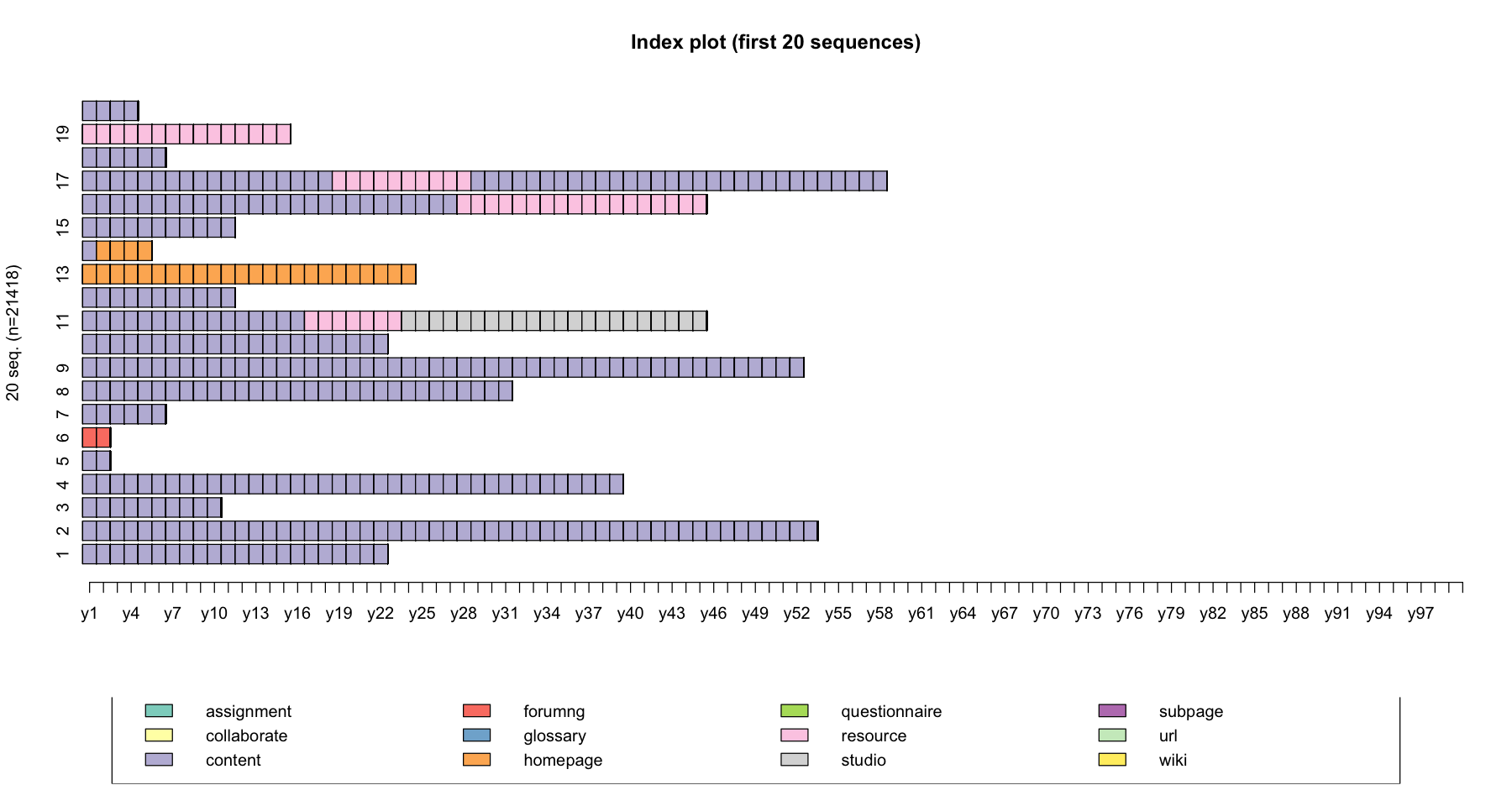
We can easily plot the top 20 sequences using the seqiplot() function.
Index plot (first 20 sequences)
seqiplot(data, main = "Index plot (first 20 sequences)", idxs = 1:20)
# Plot data during the first 100 minutes only

seqiplot(log_sts.seq[,1:100], main = "Index plot (first 20 sequences)", idxs = 1:20)
State distribution plot
The seqdplot() function plots a graphic showing the state distribution at each time point
seqdplot(data, main = "State distribution plot")
seqdplot(log_sts.seq[,1:300], main = "State distribution plot")
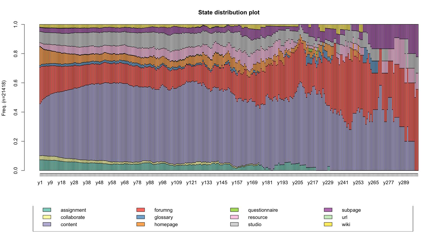
Beside plotting the distribution of the states at each time point, you may want to get the figures of the distribution. The seqstatd() function returns the table of the state distributions together with the number of valid states and an entropy measure for each time unit. We will explain what entropy means later.
Here’s I am going to return a table of state distributions of 5 time units as an example
print(seqstatd(log_sts.seq[,1:5]))
                          [State frequencies]
                  y1     y2     y3     y4     y5
assignment    0.0733 0.0732 0.0732 0.0723 0.0716
collaborate   0.0275 0.0285 0.0292 0.0291 0.0286
content       0.3562 0.3674 0.3821 0.3907 0.3981
forumng       0.2497 0.2442 0.2292 0.2217 0.2159
glossary      0.0120 0.0130 0.0144 0.0146 0.0144
homepage      0.1275 0.1142 0.1063 0.0997 0.0965
questionnaire 0.0028 0.0026 0.0023 0.0024 0.0022
resource      0.0256 0.0291 0.0325 0.0348 0.0371
studio        0.0763 0.0774 0.0788 0.0809 0.0802
subpage       0.0282 0.0286 0.0290 0.0299 0.0308
url           0.0016 0.0016 0.0017 0.0018 0.0017
wiki          0.0191 0.0203 0.0212 0.0221 0.0229

                           [Valid states]
                 y1    y2    y3    y4    y5
N             21418 21418 19605 18808 17864

                           [Entropy index]
                y1   y2   y3   y4   y5
H             0.73 0.73 0.73 0.73 0.73
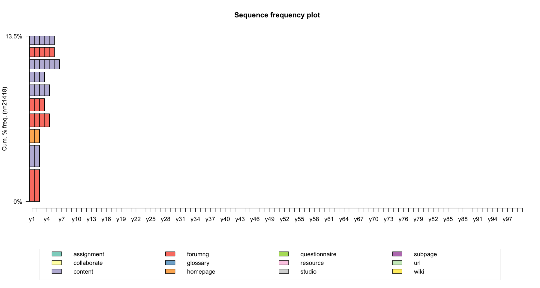
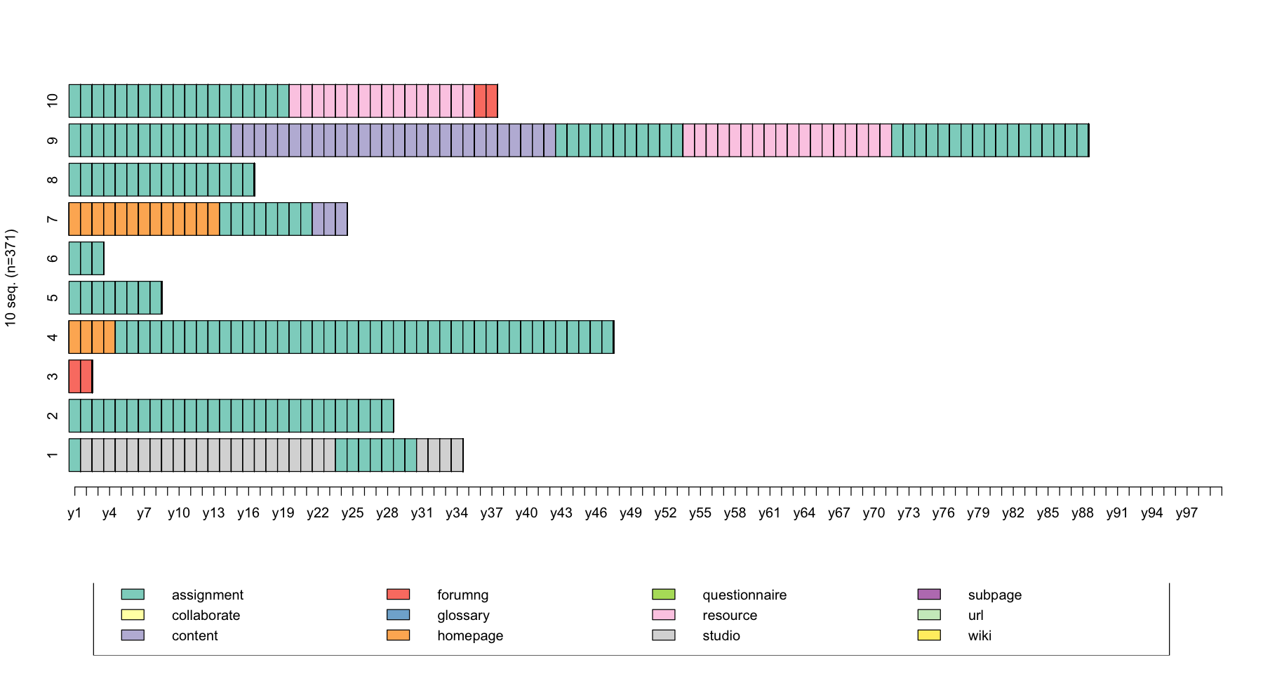
Sequence frequency plot
The seqfplot() function plots the most frequent sequences. By default, the 10 most frequent sequences are plotted. You can adjust this with the idxs option. The sequences are ordered by decreasing frequency from bottom up and the bar widths are set proportional to the sequence frequency (pbarw = TRUE)
seqfplot(data, main = "Sequence frequency plot", idxs = 1:10)
seqfplot(log_sts.seq[,1:100], main = "Sequence frequency plot", pbarw = TRUE, idxs = 1:10)
You can also return the frequency table using seqtab() function
print(seqtab(log_sts.seq[,1:100]))
           Freq Percent
forumng/2   660    3.08
content/2   440    2.05
homepage/2  273    1.27
forumng/4   270    1.26
forumng/3   256    1.20
content/4   229    1.07
content/3   207    0.97
content/6   198    0.92
forumng/5   192    0.90
content/5   177    0.83
Transition rates
The seqtrate() function computes the transition rates between states or events. The outcome is a matrix where each rows gives a transition distribution from associated originating state (or event) in t to the states in t + 1 (the figures sum to one in each row).
# ?seqtrate
seqtrate(log_sts.seq[,1:100])
[>] computing transition probabilities for states assignment/collaborate/content/forumng/glossary/homepage/questionnaire/resource/studio/subpage/url/wiki ...
| [-> assignment] | [-> collaborate] | [-> content] | [-> forumng] | [-> glossary] | [-> homepage] | [-> questionnaire] | [-> resource] | [-> studio] | [-> subpage] | [-> url] | [-> wiki] | |
|---|---|---|---|---|---|---|---|---|---|---|---|---|
| [assignment ->] | 0.954221302 | 0.0009489303 | 0.018403497 | 0.006728778 | 0.0031055901 | 0.007677709 | 2.012882e-04 | 0.0027317690 | 0.004083276 | 0.0007476421 | 2.012882e-04 | 0.0009489303 |
| [collaborate ->] | 0.003000692 | 0.9543740863 | 0.010694776 | 0.016157575 | 0.0002308225 | 0.007078557 | 0.000000e+00 | 0.0006155267 | 0.002846811 | 0.0020004616 | 7.694083e-05 | 0.0029237516 |
| [content ->] | 0.002204010 | 0.0003986776 | 0.975496372 | 0.004769087 | 0.0022378601 | 0.003148049 | 1.955777e-04 | 0.0052128976 | 0.004915770 | 0.0004663776 | 4.513331e-05 | 0.0009101885 |
| [forumng ->] | 0.001849363 | 0.0021626429 | 0.015087971 | 0.955200954 | 0.0007276182 | 0.007933059 | 1.616929e-04 | 0.0011419563 | 0.007185229 | 0.0035471385 | 1.313755e-04 | 0.0048709994 |
| [glossary ->] | 0.009110397 | 0.0005359057 | 0.061414791 | 0.007395498 | 0.9061093248 | 0.003429796 | 1.071811e-04 | 0.0048231511 | 0.005680600 | 0.0004287245 | 1.071811e-04 | 0.0008574491 |
| [homepage ->] | 0.008770458 | 0.0025161151 | 0.035824687 | 0.017277324 | 0.0012221131 | 0.920682466 | 5.271860e-04 | 0.0020368551 | 0.006086602 | 0.0030672641 | 1.917040e-04 | 0.0017972251 |
| [questionnaire ->] | 0.011677282 | 0.0000000000 | 0.058386412 | 0.016985138 | 0.0010615711 | 0.027600849 | 8.811040e-01 | 0.0000000000 | 0.002123142 | 0.0000000000 | 0.000000e+00 | 0.0010615711 |
| [resource ->] | 0.002954587 | 0.0006930512 | 0.043188036 | 0.004741930 | 0.0009848623 | 0.003136969 | 2.918111e-04 | 0.9363487142 | 0.004741930 | 0.0010213387 | 2.553347e-04 | 0.0016414372 |
| [studio ->] | 0.002443336 | 0.0007747164 | 0.025069029 | 0.012971534 | 0.0008541745 | 0.004270873 | 5.959357e-05 | 0.0020659105 | 0.948074134 | 0.0010726843 | 7.945810e-05 | 0.0022645557 |
| [subpage ->] | 0.001477833 | 0.0024630542 | 0.007991242 | 0.014012042 | 0.0001094691 | 0.006185003 | 5.473454e-05 | 0.0023535851 | 0.003612479 | 0.9599890531 | 1.094691e-04 | 0.0016420361 |
| [url ->] | 0.006339144 | 0.0000000000 | 0.031695721 | 0.017432647 | 0.0000000000 | 0.009508716 | 0.000000e+00 | 0.0110935024 | 0.004754358 | 0.0063391442 | 9.064976e-01 | 0.0063391442 |
| [wiki ->] | 0.001951805 | 0.0030778470 | 0.015614443 | 0.032880414 | 0.0010509721 | 0.005104722 | 0.000000e+00 | 0.0032279859 | 0.009008333 | 0.0020268749 | 0.000000e+00 | 0.9260566024 |
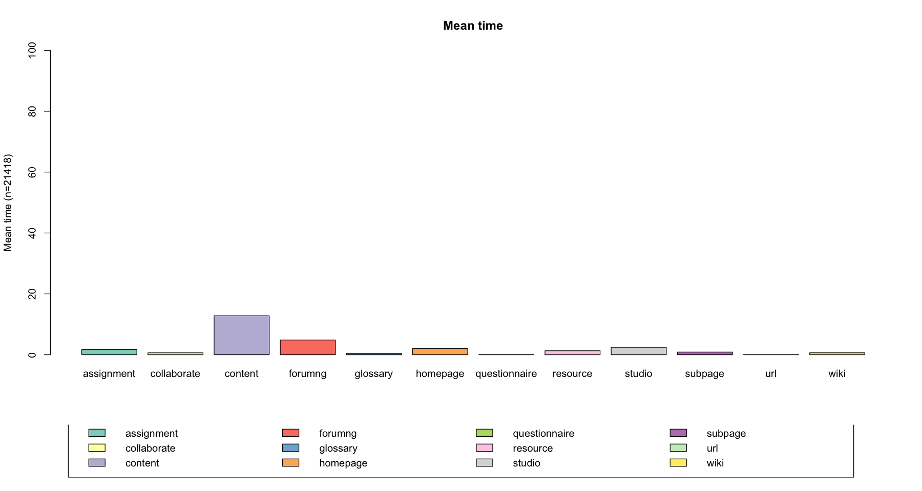
Average time spent in each state
The seqmtplot() function to visualize the mean time spent in each state. You can also create multiple plots by group using the group option.
seqmtplot(log_sts.seq[,1:100], group = NULL, title = "Mean time")
[!!] In IRkernel::main() : title is deprecated, use main instead.
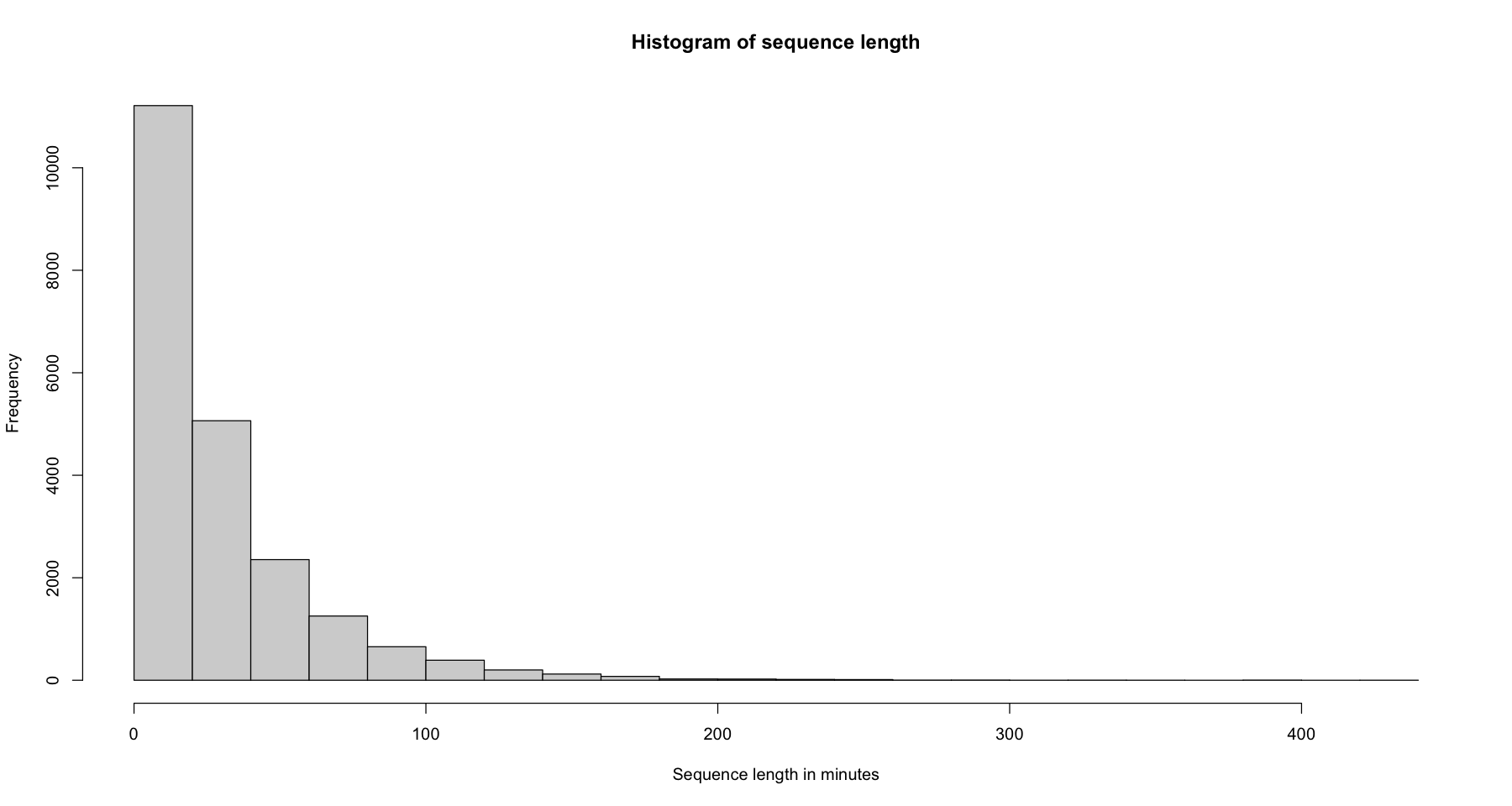
Descriptive statisitics of sequences
Sequence length using the
seqlength()function
hist(seqlength(log_sts.seq), main = 'Histogram of sequence length', xlab="Sequence length in minutes")
Distinct states sequence (DSS) using the
seqdss()function
print(seqdss(log_sts.seq[31:41,1:100]))
   Sequence
45 assignment-studio-assignment-studio
46 assignment
48 forumng
50 homepage-assignment
51 assignment
54 assignment
55 homepage-assignment-content
56 assignment
57 assignment-content-assignment-resource-assignment
59 assignment-resource-forumng
61 content
Shanon’s entropy is calculated as:
where s is the size of the alphabet
\(\pi_i\) the proportion of occurrences of the ith state in the considered sequence
The entropy can be interpreted as the ‘uncertainty’ of predicting the states in a given sequence. If all states in the sequence are the same, the entropy is equal to 0. It is maximum when the cases are equally distributed between the states
The seqient() function returns by default a normalized Shanon’s entropy
seqiplot(log_sts.seq[31:41,1:100])
seqient(log_sts.seq[31:41,1:100], norm = TRUE)
| Entropy | |
|---|---|
| 45 | 0.2195634 |
| 46 | 0.0000000 |
| 48 | 0.0000000 |
| 50 | 0.1171340 |
| 51 | 0.0000000 |
| 54 | 0.0000000 |
| 55 | 0.3856211 |
| 56 | 0.0000000 |
| 57 | 0.4193275 |
| 59 | 0.3470891 |
| 61 | 0.0000000 |

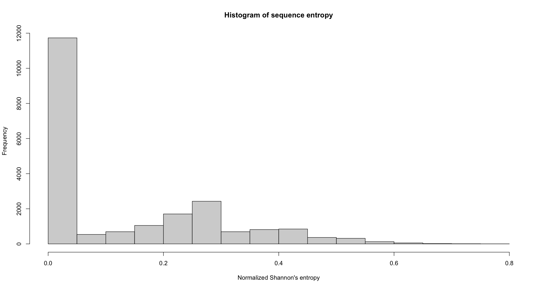
Let’s plot a histogram of entropy for the whole dataset
hist(seqient(log_sts.seq), main = 'Histogram of sequence entropy', xlab="Normalized Shannon's entropy")
Let us have a look at the sequences near the minimum, median and maximum entropy. For that, we draw sets of sequences having an entropy lower or equal to the 55th percentile, an entropy 50-90th percentile, and an entropy greater than the 90th percentile.
ient.quant <- quantile(seqient(log_sts.seq[,1:100]), c(0, 0.55, 0.9, 1))
ient.quant
- 0%
- 0
- 55%
- 0.0533989559934544
- 90%
- 0.372804151486808
- 100%
- 0.775849600937639
ient.group <- cut(seqient(log_sts.seq[,1:100]), ient.quant, labels = c("55th or lower", "55th-90th", "above 90th"), include.lowest = T)
ient.group <- factor(ient.group, levels = c("55th or lower", "55th-90th", "above 90th"))
table(ient.group)
ient.group
55th or lower     55th-90th    above 90th
        11783          7493          2142
options(repr.plot.width=15, repr.plot.height=8)
seqfplot(log_sts.seq[,1:100], group = ient.group, pbarw = TRUE)

Turbulence
The Turbulence depends on the length of the sequence. The Turbulence is based on the number \(\phi\)(x) of distinct subsequences that can be extracted from the distinct state sequence and the variance of the consecutive times ti spent in the distinct states.
seqiplot(log_sts.seq[31:401,1:100])
cbind(seqST(log_sts.seq[31:41,1:100]),seqient(log_sts.seq[31:41,1:100]))
| Turbulence | Entropy | |
|---|---|---|
| 45 | 4.942382 | 0.2195634 |
| 46 | 1.000000 | 0.0000000 |
| 48 | 1.000000 | 0.0000000 |
| 50 | 2.411960 | 0.1171340 |
| 51 | 1.000000 | 0.0000000 |
| 54 | 1.000000 | 0.0000000 |
| 55 | 5.486399 | 0.3856211 |
| 56 | 1.000000 | 0.0000000 |
| 57 | 9.603334 | 0.4193275 |
| 59 | 5.206116 | 0.3470891 |
| 61 | 1.000000 | 0.0000000 |
Finally, we can use a single function seqindic to produce multiple descriptive statistics of the sequences. Here’s a few examples
“lgth” (sequence length)
“trans” (number of state changes)
“entr” (longitudinal normalized entropy)
“cplx” (complexity index)
“turb” (turbulence)
# ?seqindic
seqindic(log_sts.seq[31:41,1:100], indic=c("lgth","trans","entr","turbn","cplx"))
| Lgth | Trans | Entr | Cplx | Turbn | |
|---|---|---|---|---|---|
| <dbl> | <dbl> | <dbl> | <dbl> | <dbl> | |
| 45 | 34 | 3 | 0.2195634 | 0.14128096 | 0.04532171 |
| 46 | 28 | 0 | 0.0000000 | 0.00000000 | 0.00000000 |
| 48 | 2 | 0 | 0.0000000 | 0.00000000 | 0.00000000 |
| 50 | 47 | 1 | 0.1171340 | 0.05046179 | 0.01623192 |
| 51 | 8 | 0 | 0.0000000 | 0.00000000 | 0.00000000 |
| 54 | 3 | 0 | 0.0000000 | 0.00000000 | 0.00000000 |
| 55 | 24 | 2 | 0.3856211 | 0.18311820 | 0.05157575 |
| 56 | 16 | 0 | 0.0000000 | 0.00000000 | 0.00000000 |
| 57 | 88 | 4 | 0.4193275 | 0.13885037 | 0.09890414 |
| 59 | 37 | 2 | 0.3470891 | 0.13886226 | 0.04835361 |
| 61 | 13 | 0 | 0.0000000 | 0.00000000 | 0.00000000 |